Filter Theory#
The theory behind gcm-filters is described here at a high level.
For a more detailed treatment, see Grooms et al. (2021).
Filter Scale and Shape#
Any low-pass spatial filter should have a target length scale such that the filtered field keeps the part of the signal with length scales larger than the target length scale, and smooths out smaller scales. In the context of this package the target length scale is called filter_scale.
A spatial filter can also have a shape that determines how sharply it separates scales above and below the target length scale. The filter shape can be thought of in terms of the kernel of a convolution filter
where \(f\) is the function being filtered, \(G\) is the filter kernel, and \(x'\) is a dummy integration variable. (We note, however, that our filter is not exactly the same as a convolution filter. So our filter with a Gaussian target does not exactly produce the same results as a convolution against a Gaussian kernel on the sphere.)
This package currently has two filter shapes: GAUSSIAN and TAPER.
In [1]: list(gcm_filters.FilterShape)
Out[1]: [<FilterShape.GAUSSIAN: 1>, <FilterShape.TAPER: 2>]
For the GAUSSIAN filter the filter_scale equals \(\sqrt{12}\times\) the standard deviation of the Gaussian.
I.e. if you want to use a Gaussian filter with standard deviation L, then you should set filter_scale equal to L \(\times\sqrt{12}\).
This strange-seeming choice makes the Gaussian kernel have the same effect on large scales as a boxcar filter of width filter_scale.
Thus filter_scale can be thought of as the “coarse grid scale” of the filtered field.
We can create a Gaussian filter as follows.
In [2]: gaussian_filter = gcm_filters.Filter(
   ...:     filter_scale=4,
   ...:     dx_min=1,
   ...:     filter_shape=gcm_filters.FilterShape.GAUSSIAN,
   ...:     grid_type=gcm_filters.GridType.REGULAR,
   ...: )
   ...:

In [3]: gaussian_filter
Out[3]: Filter(filter_scale=4, dx_min=1, filter_shape=<FilterShape.GAUSSIAN: 1>, transition_width=3.141592653589793, ndim=2, n_steps=np.int64(5), grid_type=<GridType.REGULAR: 1>)
Once the filter has been constructed, the method plot_shape can be used to plot the shape of the target filter and the approximate filter.
In [4]: gaussian_filter.plot_shape()
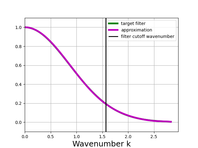
The distinction between the target filter and the approximate filter will be discussed below.
Note
plot_shape does not plot the shape of the filter kernel. Instead, it plots the frequency response of the filter for each wavenumber \(k\).
In other words, the plot shows how the filter attenuates different scales in the data.
Length scales are related to wavenumbers by \(\ell = 2\pi/k\).
The filter leaves large scales unchanged, so the plot shows values close to 1 for small \(k\).
The filter damps out small scales, so the plots shows values close to 0 for large \(k\).
The definition of the TAPER filter is more complex, but the filter_scale has the same meaning: it corresponds to the width of a qualitatively-similar boxcar filter.
In [5]: taper_filter = gcm_filters.Filter(
   ...:     filter_scale=4,
   ...:     dx_min=1,
   ...:     filter_shape=gcm_filters.FilterShape.TAPER,
   ...:     grid_type=gcm_filters.GridType.REGULAR,
   ...: )
   ...:

In [6]: taper_filter
Out[6]: Filter(filter_scale=4, dx_min=1, filter_shape=<FilterShape.TAPER: 2>, transition_width=3.141592653589793, ndim=2, n_steps=np.int64(16), grid_type=<GridType.REGULAR: 1>)
In [7]: taper_filter.plot_shape()
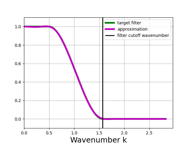
The plot above shows that the TAPER filter is more scale-selective than the Gaussian filter; it does a better job of leaving scales larger than the filter scale unchanged, and removing scales smaller than the filter scale.
The drawbacks of the TAPER filter are that it requires higher computational cost for the same filter scale (due to a higher number of necessary filter steps, see below), and it can produce negative values for the filtered field even when the unfiltered field is positive.
The Taper filter has a tunable parameter transition_width that controls how sharply the filter separates scales above and below the filter scale.
transition_width = 1 would be the same as a complete projection onto the large scales, leaving the small scales completely zeroed out.
This would require a very high computational cost, and is not at all recommended!
The default is transition_width = \(\pi\).
Larger values for transition_width reduce the cost and the likelihood of producing negative values from positive data, but make the filter less scale-selective. In the example below, we choose transition_width = \(2\pi\).
In [8]: wider_taper_filter = gcm_filters.Filter(
   ...:     filter_scale=4,
   ...:     dx_min=1,
   ...:     filter_shape=gcm_filters.FilterShape.TAPER,
   ...:     transition_width=2*np.pi,
   ...:     grid_type=gcm_filters.GridType.REGULAR,
   ...: )
   ...:

In [9]: wider_taper_filter
Out[9]: Filter(filter_scale=4, dx_min=1, filter_shape=<FilterShape.TAPER: 2>, transition_width=6.283185307179586, ndim=2, n_steps=np.int64(14), grid_type=<GridType.REGULAR: 1>)
In [10]: wider_taper_filter.plot_shape()
Note
The Taper filter is similar to the Lanczos filter.
Both are 1 for a range of large scales and 0 for a range of small scales, with a transition in between.
The difference is in the transition region: in the transition region the Lanczos filter is straight line connecting 1 and 0, while the Taper filter is a smoother cubic.
The Lanczos filter is typically described in terms of its “half-power cutoff wavelength”; the Taper filter can be similarly described.
The half-power cutoff wavelength for the Taper filter with a filter_scale of \(L\) and a transition_width of \(X\) is \(2LX/(X+1)\).
Filter Steps#
Versions of the filter before v0.3 go through several steps to produce the final filtered field. There are two different kinds of steps: Laplacian and Biharmonic steps. At each Laplacian step, the filtered field is updated using the following formula
The filtered field is initialized to \(\bar{f}=f\) and \(\Delta\) denotes a discrete Laplacian. At each Biharmonic step, the filtered field is updated using
where \(R\{\cdot\}\) denotes the real part of a complex number.
The total number of steps, n_steps, and the values of \(s_j\) are automatically selected by the code to produce the desired filter scale and shape.
If the filter scale is much larger than the grid scale, many steps are required.
Also, the Taper filter requires more steps than the Gaussian filter for the same filter_scale; in the above examples the Taper filters required n_steps = 16, but the Gaussian filter only n_steps = 5.
The code allows users to set their own n_steps.
Biharmonic steps are counted as 2 steps because their cost is approximately twice as much as a Laplacian step.
So with n_steps = 3 you might get one Laplacian plus one biharmonic step, or three Laplacian steps.
(The user cannot choose how n_steps is split between Laplacian and Biharmonic steps; that split is set internally in the code.)
For example, the user might want to use a smaller number of steps to reduce the cost. The caveat is that the accuracy will be reduced, so the filter might not act as expected: it may not have the right shape or the right length scale. To illustrate this, we create a new filter with a smaller number of steps than the default n_steps = 16, and plot the result.
In [11]: taper_filter_8steps = gcm_filters.Filter(
   ....:     filter_scale=4,
   ....:     dx_min=1,
   ....:     filter_shape=gcm_filters.FilterShape.TAPER,
   ....:     n_steps=8,
   ....:     grid_type=gcm_filters.GridType.REGULAR,
   ....: )
   ....:

In [12]: taper_filter_8steps
Out[12]: Filter(filter_scale=4, dx_min=1, filter_shape=<FilterShape.TAPER: 2>, transition_width=3.141592653589793, ndim=2, n_steps=8, grid_type=<GridType.REGULAR: 1>)
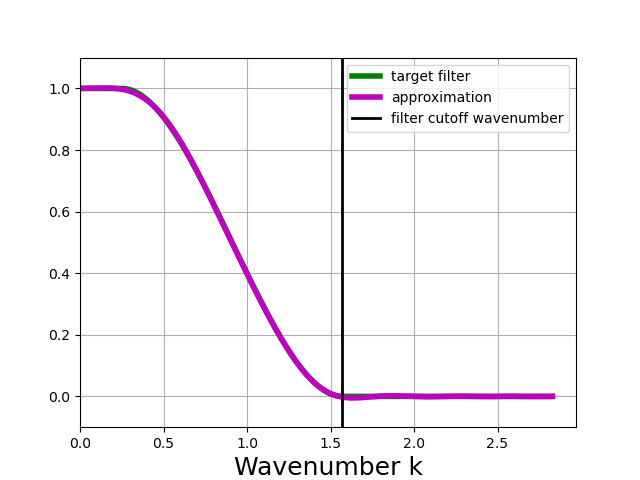
In [13]: taper_filter_8steps.plot_shape()

The example above shows that using n_steps = 8 still yields a very accurate approximation of the target filter, at half the cost of the default. The main drawback in this example is that the filter slightly amplifies large scales, which also implies that it will not conserve variance.
The example below shows what happens with n_steps = 4.
In [14]: taper_filter_4steps = gcm_filters.Filter(
   ....:     filter_scale=4,
   ....:     dx_min=1,
   ....:     filter_shape=gcm_filters.FilterShape.TAPER,
   ....:     n_steps=4,
   ....:     grid_type=gcm_filters.GridType.REGULAR,
   ....: )
   ....:

In [15]: taper_filter_4steps
Out[15]: Filter(filter_scale=4, dx_min=1, filter_shape=<FilterShape.TAPER: 2>, transition_width=3.141592653589793, ndim=2, n_steps=4, grid_type=<GridType.REGULAR: 1>)
In [16]: taper_filter_4steps.plot_shape()
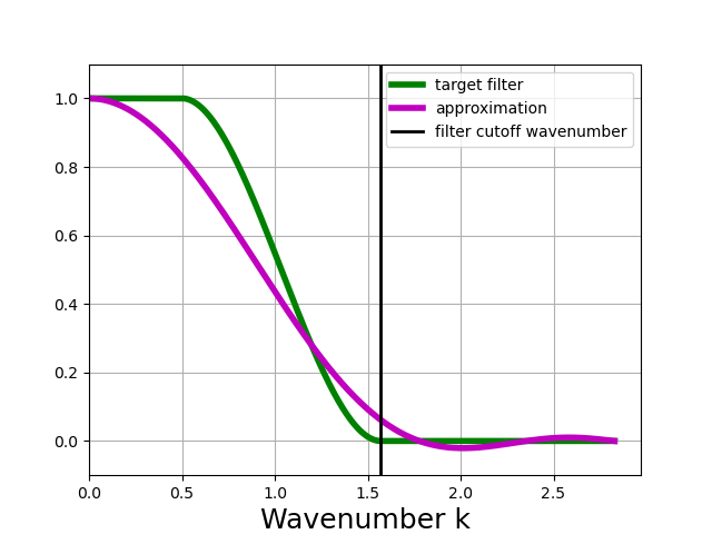
Warning
For this example of a Taper filter with a filter factor of 4, n_steps = 4 is simply not enough to get a good approximation of the target filter. The taper_filter_4steps object created here will still “work” but it will not behave as expected; specifically, it will smooth more than expected - it will act like a filter with a larger filter scale.
The minimum number of steps is 3; if n_steps is not set by the user, or if it is set to a value less than 3, the code automatically changes n_steps to the default value.
Numerical Stability and Chebyshev Algorithm#
gcm-filters approximates the target filter using a polynomial.
The foregoing section describes how the polynomial can be applied to data via a stepwise algorithm, which relies on the following representation of the polynomial
where \(-s\) corresponds to the discrete Laplacian and \(s_i\) are the roots of the polynomial. The numerical stability of this algorithm depends strongly on the ordering of the steps, i.e. of the polynomial roots. As described by Grooms et al. (2021), roundoff error can accumulate and corrupt the results, especially when the filter scale is much larger than the grid scale.
A different iterative algorithm for applying the filter to data can be formulated based on a different representation of the polynomial. The polynomial approximation is actually found using a new variable \(t\) (which does not represent time!)
and it is represented using Chebyshev coordinates \(c_i\) rather than roots \(s_i\):
where \(T_i(t)\) are Chebyshev polynomials of the first kind. Where the variable \(-s\) corresponds to the discrete Laplacian, the new variable \(t\) corresponds to a scaled and shifted Laplacian.
This suggests an alternative way of applying the filter to data. Let
be the discrete Laplacian \(\Delta\) with a rescaling and a shift. In principle one could apply the filter to a vector of data \(\mathbf{f}\) by computing the vectors \(T_i(\mathbf{A})\mathbf{f}\) and then taking a linear combination with weights \(c_i\). This begs the question of how to compute the vectors \(T_i(\mathbf{A})\mathbf{f}\).
Fortunately, this can be done using the three-term recurrence for Chebyshev polynomials. Chebyshev polynomials satisfy the following recurrence relation
This relation implies that we can evaluate the vectors \(T_i(\mathbf{A})\mathbf{f}\) using the following recurrence
In summary, the Chebyshev representation of the filter polynomial, together with the three-term recurrence for Chebyshev polynomials and a method for applying a scaled and shifted discrete Laplacian to data, result in an alternative algorithm for applying the filter to data that is different from the one described in Grooms et al. (2021). Despite being a different algorithm, in the absence of roundoff errors this will produce exactly the same result as the original algorithm. Experience has shown that the Chebyshev-based algorithm is much more stable to roundoff errors. As of version v0.3, the code uses the more stable Chebyshev-based algorithm described in this section.
Spatially-Varying Filter Scale#
In the foregoing discussion the filter scale is fixed over the physical domain. It is possible to vary the filter scale over the domain by introducing a diffusivity \(\kappa\). (This diffusivity is nondimensional.) The Laplacian steps are altered to
and the Biharmonic steps are similarly altered by replacing \(\Delta\) with \(\nabla\cdot(\kappa\nabla)\).
With \(\kappa\) the local filter scale is \(\sqrt{\kappa}\times\) filter_scale.
For reasons given in Grooms et al. (2021), we require \(\kappa\le 1\), and at least one place in the domain where \(\kappa = 1\).
Thus, when using variable \(\kappa\), filter_scale sets the largest filter scale in the domain and the local filter scale can be reduced by making \(\kappa<1\).
Suppose, for example, that you want the local filter scale to be \(L(x,y)\).
You can achieve this in gcm-filters as follows.
Set
filter_scaleequal to the maximum of \(L(x,y)\) over the domain. (Call this value \(L_{max}\)).Set \(\kappa\) equal to \(L(x,y)^2/L_{max}^2\).
Example: Different filter types has examples of filtering with spatially-varying filter scale.
Anisotropic Filtering#
It is possible to have different filter scales in different directions, and to have both the scales and directions vary over the domain.
This is achieved by replacing \(\kappa\) in the previous section with a \(2\times2\) symmetric and positive definite matrix (for a 2D domain), i.e. replacing \(\Delta\) with \(\nabla\cdot(\mathbf{K}\nabla)\).
gcm-filters currently only supports diagonal \(\mathbf{K}\), i.e. the principal axes of the anisotropic filter are aligned with the grid, so that the user only inputs one \(\kappa\) for each grid direction, rather than a full \(2\times2\) matrix.
Just like in the previous section, we require that each of these two \(\kappa\) be less than or equal to 1, and the interpretation is also the same: the local filter scale in a particular direction is \(\sqrt{\kappa}\times\) filter_scale.
Suppose, for example, that you want to filter with a scale of 60 in the grid-x direction and a scale of 30 in the grid-y direction.
Then you would set filter_scale = 60, with \(\kappa_x = 1\) to get a filter scale of 60 in the grid-x direction.
Next, to get a filter scale of 30 in the grid-y direction you would set \(\kappa_y=1/4\).
The Example: Different filter types has examples of anisotropic filtering.
Fixed Factor Filtering#
Example: Different filter types also shows methods designed specifically for the case where the user wants to set the local filter scale equal to a multiple \(m\) of the local grid scale to achieve a fixed coarsening factor. This can be achieved using the anisotropic diffusion described in the previous section.
An alternative way to achieve filtering with fixed coarsening factor \(m\) is what we refer to as simple fixed factor filtering. This method is somewhat ad hoc, and not equivalent to fixed factor filtering via anisotropic diffusion. On the upside, simple fixed factor filtering is often significantly faster and yields very similar results in practice, as seen in Example: Different filter types. The code handles simple fixed factor filtering as follows:
It multiplies the unfiltered data by the local grid cell area.
It applies a filter with
filter_scale= \(m\) as if the grid scale were uniform.It divides the resulting field by the local grid cell area.
The first step is essentially a coordinate transformation where your original (locally orthogonal) grid is transformed to a uniform Cartesian grid with \(dx = dy = 1\). The third step is the reverse coordinate transformation.
Note
The three steps above are handled internally by gcm-filters if the user chooses one of the following grid types:
REGULAR_AREA_WEIGHTEDREGULAR_WITH_LAND_AREA_WEIGHTEDTRIPOLAR_REGULAR_WITH_LAND_AREA_WEIGHTED
together with filter_scale = \(m\) and dx_min = 1. (For simple fixed factor filtering, only dx_min on the transformed uniform grid matters; and here we have dx_min = 1). Read more about the different grid types in Basic Filtering.
Filtering Vectors#
In Cartesian geometry the Laplacian of a vector field can be obtained by taking the Laplacian of each component of the vector field, so vector fields can be filtered as described in the foregoing sections. On smooth manifolds, the Laplacian of a vector field is not the same as the Laplacian of each component of the vector field. Users may wish to use a vector Laplacian to filter vector fields. The filter is constructed in exactly the same way; the only difference is in how the Laplacian is defined. Rather than taking a scalar field and returning a scalar field, the vector Laplacian takes a vector field as input and returns a vector field. To distinguish this from the scalar Laplacian, we refer to the filter based on a scalar Laplacian as a diffusion-based filter and the filter based on a vector Laplacian as a viscosity-based filter. Example: Viscosity-based filtering with vector Laplacians has examples of viscosity-based filtering.