Filtering on CPUs versus GPUs#
This tutorial gives a quick introduction to using GCM-Filters on either CPU’s or GPU’s.
import gcm_filters
import numpy as np
import xarray as xr
POP data#
We are going to work with data from the CORE-forced Parallel Ocean Program (POP) simulation described in Johnson et al. (2016). The corresponding grid is the 0.1 degree nominal resolution POP tripole grid (Smith et al., 2010). SST snapshot data and grid variables are stored in the following dataset, which we pull from figshare.
import pooch

fname = pooch.retrieve(
    url="doi:10.6084/m9.figshare.14607684.v1/POP_SST.nc",
    known_hash="md5:0023da8e42dcd2141805e553a023078c",
)
ds = xr.open_dataset(fname)
ds
<xarray.Dataset>
Dimensions:  (nlat: 2400, nlon: 3600, time: 1, z_t: 62)
Coordinates:
  * time     (time) object 0033-11-27 00:00:00
  * z_t      (z_t) float32 500.0 1.5e+03 2.5e+03 ... 5.625e+05 5.875e+05
    ULONG    (nlat, nlon) float64 ...
    ULAT     (nlat, nlon) float64 ...
    TLONG    (nlat, nlon) float64 ...
    TLAT     (nlat, nlon) float64 ...
Dimensions without coordinates: nlat, nlon
Data variables:
    KMT      (nlat, nlon) float64 ...
    TAREA    (nlat, nlon) float64 ...
    HTN      (nlat, nlon) float64 ...
    HTE      (nlat, nlon) float64 ...
    HUS      (nlat, nlon) float64 ...
    HUW      (nlat, nlon) float64 ...
    SST      (time, nlat, nlon) float32 ...
Attributes:
    title:           g.e01.GIAF.T62_t12.003
    history:         none
    Conventions:     CF-1.0; http://www.cgd.ucar.edu/cms/eaton/netcdf/CF-curr...
    contents:        Diagnostic and Prognostic Variables
    source:          CCSM POP2, the CCSM Ocean Component
    revision:        $Id: tavg.F90 46405 2013-04-26 05:24:34Z mlevy@ucar.edu $
    calendar:        All years have exactly  365 days.
    start_time:      This dataset was created on 2014-07-19 at 17:28:03.3
    cell_methods:    cell_methods = time: mean ==> the variable values are av...
    nsteps_total:    9618241
    tavg_sum:        431999.9999999717
tavg_sum_qflux: 432000.00000000006In this example, we want to filter SST with a fixed factor of 10, i.e., to nominally 1 degree resolution.
To keep things simple, we will filter with the simple fixed factor filter. The TRIPOLAR_REGULAR_WITH_LAND_AREA_WEIGHTED Laplacian is suitable for this filter and our data on a tripole grid. This Laplacian only needs the grid cell area and wet_mask as grid input variables.
gcm_filters.required_grid_vars(gcm_filters.GridType.TRIPOLAR_REGULAR_WITH_LAND_AREA_WEIGHTED)
['area', 'wet_mask']
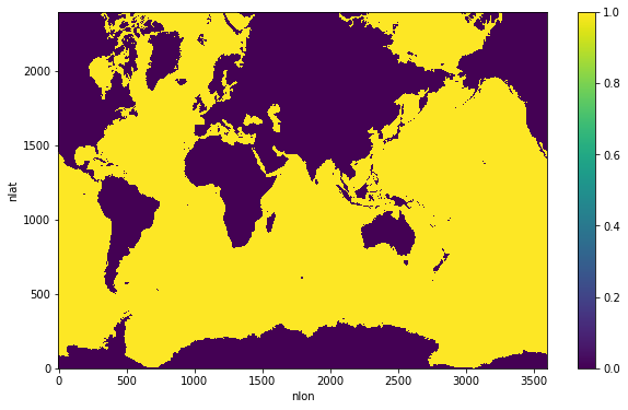
wet_mask is a mask that is 1 in ocean T-cells, and 0 in land T-cells. Since we only want to filter temperature in the uppermost level, we only need a 2D wet_mask.
wet_mask = xr.where(ds['KMT']>0, 1, 0)
wet_mask.plot(figsize=(10,6), cbar_kwargs={'label': ''});
/glade/work/noraloose/my_npl_clone/lib/python3.7/site-packages/xarray/plot/plot.py:1445: FutureWarning: Conversion of the second argument of issubdtype from `str` to `str` is deprecated. In future, it will be treated as `np.str_ == np.dtype(str).type`.
  and not np.issubdtype(x.dtype, str)
/glade/work/noraloose/my_npl_clone/lib/python3.7/site-packages/xarray/plot/plot.py:1460: FutureWarning: Conversion of the second argument of issubdtype from `str` to `str` is deprecated. In future, it will be treated as `np.str_ == np.dtype(str).type`.
  and not np.issubdtype(y.dtype, str)
The area of the T-cells is
area = ds.TAREA / 10000 # convert units from cm2 to m2
Filtering on CPUs#
We tell gcm-filters to filter on CPU’s by providing a wet_mask and input data that are NumPy Arrays or Dask Arrays with NumPy chunks (rather than CuPy Arrays or Dask Arrays with CuPy chunks).
wet_mask = wet_mask.chunk({'nlat': len(ds.nlat), 'nlon': len(ds.nlon)})  # 1 chunk
wet_mask
<xarray.DataArray 'KMT' (nlat: 2400, nlon: 3600)>
dask.array<xarray-<this-array>, shape=(2400, 3600), dtype=int64, chunksize=(2400, 3600), chunktype=numpy.ndarray>
Coordinates:
    ULONG    (nlat, nlon) float64 dask.array<chunksize=(2400, 3600), meta=np.ndarray>
    ULAT     (nlat, nlon) float64 dask.array<chunksize=(2400, 3600), meta=np.ndarray>
    TLONG    (nlat, nlon) float64 dask.array<chunksize=(2400, 3600), meta=np.ndarray>
    TLAT     (nlat, nlon) float64 dask.array<chunksize=(2400, 3600), meta=np.ndarray>
Dimensions without coordinates: nlat, nlonarea = area.chunk({'nlat': len(ds.nlat), 'nlon': len(ds.nlon)}) # 1 chunk
area
<xarray.DataArray 'TAREA' (nlat: 2400, nlon: 3600)>
dask.array<xarray-<this-array>, shape=(2400, 3600), dtype=float64, chunksize=(2400, 3600), chunktype=numpy.ndarray>
Coordinates:
    ULONG    (nlat, nlon) float64 dask.array<chunksize=(2400, 3600), meta=np.ndarray>
    ULAT     (nlat, nlon) float64 dask.array<chunksize=(2400, 3600), meta=np.ndarray>
    TLONG    (nlat, nlon) float64 dask.array<chunksize=(2400, 3600), meta=np.ndarray>
    TLAT     (nlat, nlon) float64 dask.array<chunksize=(2400, 3600), meta=np.ndarray>
Dimensions without coordinates: nlat, nlonsst = ds.SST.where(wet_mask)
sst = sst.chunk({'nlat': len(ds.nlat), 'nlon': len(ds.nlon)}) # 1 chunk
sst
<xarray.DataArray 'SST' (time: 1, nlat: 2400, nlon: 3600)>
dask.array<where, shape=(1, 2400, 3600), dtype=float32, chunksize=(1, 2400, 3600), chunktype=numpy.ndarray>
Coordinates:
  * time     (time) object 0033-11-27 00:00:00
    ULONG    (nlat, nlon) float64 dask.array<chunksize=(2400, 3600), meta=np.ndarray>
    ULAT     (nlat, nlon) float64 dask.array<chunksize=(2400, 3600), meta=np.ndarray>
    TLONG    (nlat, nlon) float64 dask.array<chunksize=(2400, 3600), meta=np.ndarray>
    TLAT     (nlat, nlon) float64 dask.array<chunksize=(2400, 3600), meta=np.ndarray>
Dimensions without coordinates: nlat, nlon
Attributes:
    units:      degC
long_name: Surface Potential TemperatureThese are our filter specs (see also the section on simple fixed factor filters in this tutorial):
specs = {
    'filter_scale': 10,
    'dx_min': 1,
    'filter_shape': gcm_filters.FilterShape.GAUSSIAN,
    'grid_type': gcm_filters.GridType.TRIPOLAR_REGULAR_WITH_LAND_AREA_WEIGHTED
}
We now create our CPU-compatible filter with our NumPy-based area and wet_mask.
filter_cpu = gcm_filters.Filter(grid_vars={'area': area, 'wet_mask': wet_mask}, **specs)
filter_cpu
Filter(filter_scale=10, dx_min=1, filter_shape=<FilterShape.GAUSSIAN: 1>, transition_width=3.141592653589793, ndim=2, n_steps=11, grid_type=<GridType.TRIPOLAR_REGULAR_WITH_LAND_AREA_WEIGHTED: 8>)
Next, we filter the NumPy-based SST lazily on the CPU’s with the simple fixed factor filter.
filtered_cpu = filter_cpu.apply(sst, dims=['nlat', 'nlon'])
filtered_cpu
<xarray.DataArray (time: 1, nlat: 2400, nlon: 3600)>
dask.array<transpose, shape=(1, 2400, 3600), dtype=float32, chunksize=(1, 2400, 3600), chunktype=numpy.ndarray>
Coordinates:
  * time     (time) object 0033-11-27 00:00:00
    ULONG    (nlat, nlon) float64 -1.0 -1.0 -1.0 -1.0 ... -1.0 -1.0 -1.0 -1.0
    ULAT     (nlat, nlon) float64 -1.0 -1.0 -1.0 -1.0 ... -1.0 -1.0 -1.0 -1.0
    TLONG    (nlat, nlon) float64 -1.0 -1.0 -1.0 -1.0 ... -1.0 -1.0 -1.0 -1.0
    TLAT     (nlat, nlon) float64 -1.0 -1.0 -1.0 -1.0 ... -1.0 -1.0 -1.0 -1.0
Dimensions without coordinates: nlat, nlonNothing has actually been computed yet. Let’s trigger computation.
%time filtered_cpu = filtered_cpu.compute()
CPU times: user 3.34 s, sys: 1.86 s, total: 5.2 s
Wall time: 5.21 s
Here is a comparison of unfiltered vs. filtered SST, zoomed into the Gulf Stream region.
import matplotlib.pyplot as plt

vmin = 5
vmax = 25
yslice = slice(1500, 1750)
xslice = slice(400, 600)

fig,axs = plt.subplots(1,2,figsize=(25,7))
sst.isel(nlat=yslice, nlon=xslice).plot(
    ax=axs[0],
    vmin=vmin, vmax=vmax,
    cbar_kwargs={'label': 'degC'}
)
axs[0].set_title('SST', fontsize=18)
filtered_cpu.isel(nlat=yslice, nlon=xslice).plot(
    ax=axs[1],
    vmin=vmin, vmax=vmax,
    cbar_kwargs={'label': 'degC'}
)
axs[1].set_title('filtered SST (on CPU)', fontsize=18);
/glade/work/noraloose/my_npl_clone/lib/python3.7/site-packages/xarray/plot/plot.py:1445: FutureWarning: Conversion of the second argument of issubdtype from `str` to `str` is deprecated. In future, it will be treated as `np.str_ == np.dtype(str).type`.
  and not np.issubdtype(x.dtype, str)
/glade/work/noraloose/my_npl_clone/lib/python3.7/site-packages/xarray/plot/plot.py:1460: FutureWarning: Conversion of the second argument of issubdtype from `str` to `str` is deprecated. In future, it will be treated as `np.str_ == np.dtype(str).type`.
  and not np.issubdtype(y.dtype, str)

Filtering on GPUs#
We tell gcm-filters to filter on GPU’s by providing a wet_mask and input data that are CuPy Arrays or Dask Arrays with CuPy chunks. We therefore have to map the NumPy chunks to CuPy chunks.
import cupy as cp
wet_mask_gpu = wet_mask.copy()
wet_mask_gpu.data = wet_mask_gpu.data.map_blocks(cp.asarray)
wet_mask_gpu
<xarray.DataArray 'KMT' (nlat: 2400, nlon: 3600)>
dask.array<asarray, shape=(2400, 3600), dtype=int64, chunksize=(2400, 3600), chunktype=cupy.ndarray>
Coordinates:
    ULONG    (nlat, nlon) float64 dask.array<chunksize=(2400, 3600), meta=np.ndarray>
    ULAT     (nlat, nlon) float64 dask.array<chunksize=(2400, 3600), meta=np.ndarray>
    TLONG    (nlat, nlon) float64 dask.array<chunksize=(2400, 3600), meta=np.ndarray>
    TLAT     (nlat, nlon) float64 dask.array<chunksize=(2400, 3600), meta=np.ndarray>
Dimensions without coordinates: nlat, nlonsst_gpu = sst.copy()
sst_gpu.data = sst_gpu.data.map_blocks(cp.asarray)
sst_gpu
<xarray.DataArray 'SST' (time: 1, nlat: 2400, nlon: 3600)>
dask.array<asarray, shape=(1, 2400, 3600), dtype=float32, chunksize=(1, 2400, 3600), chunktype=cupy.ndarray>
Coordinates:
  * time     (time) object 0033-11-27 00:00:00
    ULONG    (nlat, nlon) float64 dask.array<chunksize=(2400, 3600), meta=np.ndarray>
    ULAT     (nlat, nlon) float64 dask.array<chunksize=(2400, 3600), meta=np.ndarray>
    TLONG    (nlat, nlon) float64 dask.array<chunksize=(2400, 3600), meta=np.ndarray>
    TLAT     (nlat, nlon) float64 dask.array<chunksize=(2400, 3600), meta=np.ndarray>
Dimensions without coordinates: nlat, nlon
Attributes:
    units:      degC
long_name: Surface Potential Temperaturearea_gpu = area.copy()
area_gpu.data = area_gpu.data.map_blocks(cp.asarray)
area_gpu
<xarray.DataArray 'TAREA' (nlat: 2400, nlon: 3600)>
dask.array<asarray, shape=(2400, 3600), dtype=float64, chunksize=(2400, 3600), chunktype=cupy.ndarray>
Coordinates:
    ULONG    (nlat, nlon) float64 dask.array<chunksize=(2400, 3600), meta=np.ndarray>
    ULAT     (nlat, nlon) float64 dask.array<chunksize=(2400, 3600), meta=np.ndarray>
    TLONG    (nlat, nlon) float64 dask.array<chunksize=(2400, 3600), meta=np.ndarray>
    TLAT     (nlat, nlon) float64 dask.array<chunksize=(2400, 3600), meta=np.ndarray>
Dimensions without coordinates: nlat, nlonWe create the filter with the same filter specs as above, but now with CuPy-based area and wet_mask.
filter_gpu = gcm_filters.Filter(grid_vars={'area': area_gpu, 'wet_mask': wet_mask_gpu}, **specs)
filter_gpu
Filter(filter_scale=10, dx_min=1, filter_shape=<FilterShape.GAUSSIAN: 1>, transition_width=3.141592653589793, ndim=2, n_steps=11, grid_type=<GridType.TRIPOLAR_REGULAR_WITH_LAND_AREA_WEIGHTED: 8>)
Filtering of the data works the same way as before, except that we apply our filter to our CuPy-based SST.
filtered_gpu = filter_gpu.apply(sst_gpu, dims=['nlat', 'nlon'])
filtered_gpu
<xarray.DataArray (time: 1, nlat: 2400, nlon: 3600)>
dask.array<transpose, shape=(1, 2400, 3600), dtype=float32, chunksize=(1, 2400, 3600), chunktype=cupy.ndarray>
Coordinates:
  * time     (time) object 0033-11-27 00:00:00
    ULONG    (nlat, nlon) float64 -1.0 -1.0 -1.0 -1.0 ... -1.0 -1.0 -1.0 -1.0
    ULAT     (nlat, nlon) float64 -1.0 -1.0 -1.0 -1.0 ... -1.0 -1.0 -1.0 -1.0
    TLONG    (nlat, nlon) float64 -1.0 -1.0 -1.0 -1.0 ... -1.0 -1.0 -1.0 -1.0
    TLAT     (nlat, nlon) float64 -1.0 -1.0 -1.0 -1.0 ... -1.0 -1.0 -1.0 -1.0
Dimensions without coordinates: nlat, nlonIn the next cell, we map the CuPy blocks back to NumPy blocks.
filtered_gpu.data = filtered_gpu.data.map_blocks(cp.asnumpy)
filtered_gpu
<xarray.DataArray (time: 1, nlat: 2400, nlon: 3600)>
dask.array<asnumpy, shape=(1, 2400, 3600), dtype=float32, chunksize=(1, 2400, 3600), chunktype=numpy.ndarray>
Coordinates:
  * time     (time) object 0033-11-27 00:00:00
    ULONG    (nlat, nlon) float64 -1.0 -1.0 -1.0 -1.0 ... -1.0 -1.0 -1.0 -1.0
    ULAT     (nlat, nlon) float64 -1.0 -1.0 -1.0 -1.0 ... -1.0 -1.0 -1.0 -1.0
    TLONG    (nlat, nlon) float64 -1.0 -1.0 -1.0 -1.0 ... -1.0 -1.0 -1.0 -1.0
    TLAT     (nlat, nlon) float64 -1.0 -1.0 -1.0 -1.0 ... -1.0 -1.0 -1.0 -1.0
Dimensions without coordinates: nlat, nlonFiltering on GPU is quite a bit faster than on CPU above.
%time filtered_gpu = filtered_gpu.compute()
CPU times: user 3.67 s, sys: 218 ms, total: 3.89 s
Wall time: 4.5 s
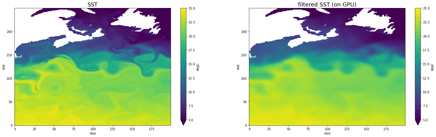
Plotting filtered SST gives the same plot as above (that’s good!).
fig,axs = plt.subplots(1,2,figsize=(25,7))
sst.isel(nlat=yslice, nlon=xslice).plot(
    ax=axs[0],
    vmin=vmin, vmax=vmax,
    cbar_kwargs={'label': 'degC'}
)
axs[0].set_title('SST', fontsize=18)
filtered_gpu.isel(nlat=yslice, nlon=xslice).plot(
    ax=axs[1],
    vmin=vmin, vmax=vmax,
    cbar_kwargs={'label': 'degC'}
)
axs[1].set_title('filtered SST (on GPU)', fontsize=18);
/glade/work/noraloose/my_npl_clone/lib/python3.7/site-packages/xarray/plot/plot.py:1445: FutureWarning: Conversion of the second argument of issubdtype from `str` to `str` is deprecated. In future, it will be treated as `np.str_ == np.dtype(str).type`.
  and not np.issubdtype(x.dtype, str)
/glade/work/noraloose/my_npl_clone/lib/python3.7/site-packages/xarray/plot/plot.py:1460: FutureWarning: Conversion of the second argument of issubdtype from `str` to `str` is deprecated. In future, it will be treated as `np.str_ == np.dtype(str).type`.
  and not np.issubdtype(y.dtype, str)
Finally, we convince ourselves that the differences in the CPU- vs. GPU-filtered fields are as small as machine precision.
fig,axs = plt.subplots(1,2,figsize=(25,7))
(filtered_cpu-filtered_gpu).plot(
    ax=axs[0],
    cbar_kwargs={'label': 'degC'}
)
axs[0].set_title('Difference: CPU-filtered - GPU-filtered', fontsize=18)
(filtered_cpu-filtered_gpu).isel(nlat=yslice, nlon=xslice).plot(
    ax=axs[1],
    cbar_kwargs={'label': 'degC'}
)
axs[1].set_title('Difference in Gulf Stream region', fontsize=18);
/glade/work/noraloose/my_npl_clone/lib/python3.7/site-packages/xarray/plot/plot.py:1445: FutureWarning: Conversion of the second argument of issubdtype from `str` to `str` is deprecated. In future, it will be treated as `np.str_ == np.dtype(str).type`.
  and not np.issubdtype(x.dtype, str)
/glade/work/noraloose/my_npl_clone/lib/python3.7/site-packages/xarray/plot/plot.py:1460: FutureWarning: Conversion of the second argument of issubdtype from `str` to `str` is deprecated. In future, it will be treated as `np.str_ == np.dtype(str).type`.
  and not np.issubdtype(y.dtype, str)
