Example: Different filter types

In this tutorial, we are going to cover how to use gcm-filters for different filter types:

• Filters with fixed filter length scale

• Filters with spatially-varying filter length scale

• Anisotropic filters

• Filters with fixed filtering factor

import gcm_filters
import numpy as np
import xarray as xr

Loading the data

In our example, we are going to use NeverWorld2 data, created by the Ocean Eddy Climate Process Team. NeverWorld2 is a regional MOM6 simulation in stacked shallow water mode, on a spherical grid. The data are stored in the cloud, on the Open Storage Network (OSN).

from intake import open_catalog
cat = open_catalog('https://raw.githubusercontent.com/ocean-eddy-cpt/cpt-data/master/catalog.yaml')
list(cat)

['neverworld_five_day_averages',
 'neverworld_quarter_degree_snapshots',
 'neverworld_quarter_degree_averages',
 'neverworld_quarter_degree_static',
 'neverworld_quarter_degree_stats',
 'neverworld_eighth_degree_snapshots',
 'neverworld_eighth_degree_averages',
 'neverworld_eighth_degree_static',
 'neverworld_eighth_degree_stats',
 'neverworld_sixteenth_degree_snapshots',
 'neverworld_sixteenth_degree_averages',
 'neverworld_sixteenth_degree_static',
 'neverworld_sixteenth_degree_stats']

In this example, we are working with 5-day averages from the 1/4 degree simulation.

ds = cat['neverworld_quarter_degree_averages'].to_dask()
ds

<xarray.Dataset>
Dimensions:     (nv: 2, time: 100, xh: 240, xq: 241, yh: 560, yq: 561, zi: 16, zl: 15)
Coordinates:
  * nv          (nv) float64 1.0 2.0
  * time        (time) object 0084-05-03 12:00:00 ... 0085-09-18 12:00:00
  * xh          (xh) float64 0.125 0.375 0.625 0.875 ... 59.12 59.38 59.62 59.88
  * xq          (xq) float64 0.0 0.25 0.5 0.75 1.0 ... 59.25 59.5 59.75 60.0
  * yh          (yh) float64 -69.88 -69.62 -69.38 -69.12 ... 69.38 69.62 69.88
  * yq          (yq) float64 -70.0 -69.75 -69.5 -69.25 ... 69.25 69.5 69.75 70.0
  * zi          (zi) float64 1.022e+03 1.023e+03 ... 1.028e+03 1.028e+03
  * zl          (zl) float64 1.023e+03 1.023e+03 ... 1.028e+03 1.028e+03
Data variables: (12/33)
    CAu         (time, zl, yh, xq) float32 dask.array<chunksize=(10, 15, 560, 241), meta=np.ndarray>
    CAv         (time, zl, yq, xh) float32 dask.array<chunksize=(10, 15, 561, 240), meta=np.ndarray>
    KE          (time, zl, yh, xh) float32 dask.array<chunksize=(10, 15, 560, 240), meta=np.ndarray>
    KE_BT       (time, zl, yh, xh) float32 dask.array<chunksize=(10, 15, 560, 240), meta=np.ndarray>
    KE_CorAdv   (time, zl, yh, xh) float32 dask.array<chunksize=(10, 15, 560, 240), meta=np.ndarray>
    KE_adv      (time, zl, yh, xh) float32 dask.array<chunksize=(10, 15, 560, 240), meta=np.ndarray>
    ...          ...
    u           (time, zl, yh, xq) float32 dask.array<chunksize=(10, 15, 560, 241), meta=np.ndarray>
    u_BT_accel  (time, zl, yh, xq) float32 dask.array<chunksize=(10, 15, 560, 241), meta=np.ndarray>
    uh          (time, zl, yh, xq) float32 dask.array<chunksize=(10, 15, 560, 241), meta=np.ndarray>
    v           (time, zl, yq, xh) float32 dask.array<chunksize=(10, 15, 561, 240), meta=np.ndarray>
    v_BT_accel  (time, zl, yq, xh) float32 dask.array<chunksize=(10, 15, 561, 240), meta=np.ndarray>
    vh          (time, zl, yq, xh) float32 dask.array<chunksize=(10, 15, 561, 240), meta=np.ndarray>
Attributes:
    associated_files:  area_t: static.nc
    filename:          averages_00030002.nc
    grid_tile:         N/A
    grid_type:         regular
    title:             NeverWorld2

Our filters also need to know about the grid that the data live on. The grid variables are stored in a separate dataset.

ds_static = cat['neverworld_quarter_degree_static'].to_dask()
ds_static

<xarray.Dataset>
Dimensions:      (time: 1, xh: 240, xq: 241, yh: 560, yq: 561)
Coordinates:
  * time         (time) object 0001-01-01 00:00:00
  * xh           (xh) float64 0.125 0.375 0.625 0.875 ... 59.38 59.62 59.88
  * xq           (xq) float64 0.0 0.25 0.5 0.75 1.0 ... 59.25 59.5 59.75 60.0
  * yh           (yh) float64 -69.88 -69.62 -69.38 -69.12 ... 69.38 69.62 69.88
  * yq           (yq) float64 -70.0 -69.75 -69.5 -69.25 ... 69.5 69.75 70.0
Data variables: (12/21)
    Coriolis     (yq, xq) float32 dask.array<chunksize=(561, 241), meta=np.ndarray>
    area_t       (yh, xh) float64 dask.array<chunksize=(560, 240), meta=np.ndarray>
    area_u       (yh, xq) float64 dask.array<chunksize=(560, 241), meta=np.ndarray>
    area_v       (yq, xh) float64 dask.array<chunksize=(561, 240), meta=np.ndarray>
    depth_ocean  (yh, xh) float32 dask.array<chunksize=(560, 240), meta=np.ndarray>
    dxCu         (yh, xq) float64 dask.array<chunksize=(560, 241), meta=np.ndarray>
    ...           ...
    geolon_u     (yh, xq) float32 dask.array<chunksize=(560, 241), meta=np.ndarray>
    geolon_v     (yq, xh) float32 dask.array<chunksize=(561, 240), meta=np.ndarray>
    wet          (yh, xh) float64 dask.array<chunksize=(560, 240), meta=np.ndarray>
    wet_c        (yq, xq) float32 dask.array<chunksize=(561, 241), meta=np.ndarray>
    wet_u        (yh, xq) float32 dask.array<chunksize=(560, 241), meta=np.ndarray>
    wet_v        (yq, xh) float32 dask.array<chunksize=(561, 240), meta=np.ndarray>
Attributes:
    filename:   static.nc
    grid_tile:  N/A
    grid_type:  regular
    title:      NeverWorld2

Filtering with fixed filter length scale

First, we filter our data with a fixed filter length scale of 200 km. That is, we use a filter that attempts to remove scales smaller than 200 km.

filter_scale = 200000

To filter our NeverWorld2 data with fixed filter length scale, we will use the grid type IRREGULAR_WITH_LAND. This grid type and its associated Laplacian work for any grid with locally orthogonal coordinates. The Laplacian needs the following grid variables:

gcm_filters.required_grid_vars(gcm_filters.GridType.IRREGULAR_WITH_LAND)

['wet_mask', 'dxw', 'dyw', 'dxs', 'dys', 'area', 'kappa_w', 'kappa_s']

Preparing the grid input variables

MOM6 uses an Arakawa C grid staggering of variables. In this tutorial, we will filter kinetic energy KE: a field that is defined at T-points (or tracer points). Note that the IRREGULAR_WITH_LAND could also be used to filter U-fields or V-fields on a C-grid (or to filter fields on a B-grid), but we would have to create the filter with different arguments for wet_mask, dxw, dyw, dxs, dys, area.

wet_mask and area are directly available from our model output:

wet_mask = ds_static.wet
area = ds_static.area_t

For the remaining grid variables, recall the following conventions:

• dxw = x-spacing centered at western cell edge

• dyw = y-spacing centered at western cell edge

• dxs = x-spacing centered at southern cell edge

• dys = y-spacing centered at southern cell edge

We get these grid variables from our model output as follows:

dxw = xr.DataArray(
    data=ds_static.dxCu.isel(xq=slice(0,-1)), 
    coords={'yh':ds.yh,'xh':ds.xh}, 
    dims=('yh','xh')
)
dyw = xr.DataArray(
    data=ds_static.dyCu.isel(xq=slice(0,-1)), 
    coords={'yh':ds.yh,'xh':ds.xh}, 
    dims=('yh','xh')
)
dxs = xr.DataArray(
    data=ds_static.dxCv.isel(yq=slice(0,-1)), 
    coords={'yh':ds.yh,'xh':ds.xh}, 
    dims=('yh','xh')
)
dys = xr.DataArray(
    data=ds_static.dyCv.isel(yq=slice(0,-1)), 
    coords={'yh':ds.yh,'xh':ds.xh}, 
    dims=('yh','xh')
)

For each grid variable in the cell above, we 1) removed the padding in the xq and yq dimensions (on the upper side) and 2) renamed the xq and yq dimensions so that all grid variables have the same dimensions: xh, yh. This is because, as of now, gcm-filters requires all input variables to have the same dimensions, even though the grid variables are assumed staggered. (This is something we would like to change in the future.)

Let’s plot a summary of the grid variables that are inputs to our filter.

import matplotlib.pyplot as plt
import matplotlib.pylab as pylab
params = {'font.size': 14}
pylab.rcParams.update(params)

fig,axs = plt.subplots(2,3,figsize=(25,15))
wet_mask.plot(ax=axs[0,0], cbar_kwargs={'label': ''})
axs[0,0].set(title='wet_mask', xlabel='')
dxw.plot(ax=axs[0,1], cbar_kwargs={'label': 'm'})
axs[0,1].set(title='dxw', xlabel='', ylabel='')
dyw.plot(ax=axs[0,2], cbar_kwargs={'label': 'm'})
axs[0,2].set(title='dyw', xlabel='', ylabel='')
dxs.plot(ax=axs[1,0], cbar_kwargs={'label': 'm'})
axs[1,0].set(title='dxs')
dys.plot(ax=axs[1,1], cbar_kwargs={'label': 'm'})
axs[1,1].set(title='dys', ylabel='')
area.plot(ax=axs[1,2], cbar_kwargs={'label': 'm2'})
axs[1,2].set(title='area', ylabel='');

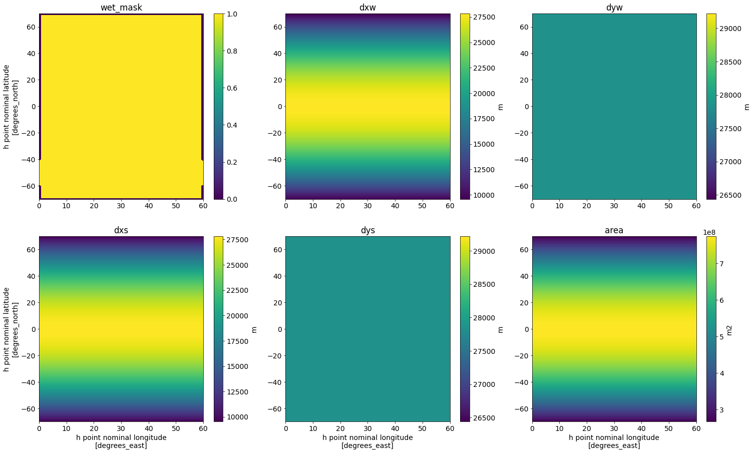
The filter needs to know what the minimum grid spacing is in our model.

dx_min = min(dxw.min(),dyw.min(),dxs.min(),dys.min())
dx_min = dx_min.values
dx_min

array(9518.17259783)

Finally, we have to set kappa_w and kappa_s. Since we don’t want to vary the filter scale spatially, we set them equal to 1 over the full domain.

kappa_w = xr.ones_like(dxw)
kappa_s = xr.ones_like(dxw)

Filtering kinetic energy

We are now ready to create our filter.

filter_200km = gcm_filters.Filter(
    filter_scale=filter_scale,
    dx_min=dx_min,
    filter_shape=gcm_filters.FilterShape.GAUSSIAN,
    grid_type=gcm_filters.GridType.IRREGULAR_WITH_LAND,
    grid_vars={
        'wet_mask': wet_mask, 
        'dxw': dxw, 'dyw': dyw, 'dxs': dxs, 'dys': dys, 'area': area, 
        'kappa_w': kappa_w, 'kappa_s': kappa_s
    }
)
filter_200km

Filter(filter_scale=200000, dx_min=array(9518.17259783), filter_shape=<FilterShape.GAUSSIAN: 1>, transition_width=3.141592653589793, ndim=2, n_steps=24, grid_type=<GridType.IRREGULAR_WITH_LAND: 5>)

We will apply the filter to ds.KE, which is a Dask array.

ds.KE

<xarray.DataArray 'KE' (time: 100, zl: 15, yh: 560, xh: 240)>
dask.array<open_dataset-22a52b531a9ba2f3287b3b412b44bd3fKE, shape=(100, 15, 560, 240), dtype=float32, chunksize=(10, 15, 560, 240), chunktype=numpy.ndarray>
Coordinates:
  * time     (time) object 0084-05-03 12:00:00 ... 0085-09-18 12:00:00
  * xh       (xh) float64 0.125 0.375 0.625 0.875 ... 59.12 59.38 59.62 59.88
  * yh       (yh) float64 -69.88 -69.62 -69.38 -69.12 ... 69.38 69.62 69.88
  * zl       (zl) float64 1.023e+03 1.023e+03 1.023e+03 ... 1.028e+03 1.028e+03
Attributes:
    cell_measures:  area: area_t
    cell_methods:   area:mean zl:mean yh:mean xh:mean time: mean
    long_name:      Layer kinetic energy per unit mass
    time_avg_info:  average_T1,average_T2,average_DT
    units:          m2 s-2

Below, we will only be interested in plotting the filtered data from a single time slice and a single layer. We can therefore make things more efficient if we first rechunk our Dask array in such a way that each chunk contains only a 2D field.

ds['KE'] = ds['KE'].chunk({'time': 1, 'zl': 1})
ds.KE

<xarray.DataArray 'KE' (time: 100, zl: 15, yh: 560, xh: 240)>
dask.array<rechunk-merge, shape=(100, 15, 560, 240), dtype=float32, chunksize=(1, 1, 560, 240), chunktype=numpy.ndarray>
Coordinates:
  * time     (time) object 0084-05-03 12:00:00 ... 0085-09-18 12:00:00
  * xh       (xh) float64 0.125 0.375 0.625 0.875 ... 59.12 59.38 59.62 59.88
  * yh       (yh) float64 -69.88 -69.62 -69.38 -69.12 ... 69.38 69.62 69.88
  * zl       (zl) float64 1.023e+03 1.023e+03 1.023e+03 ... 1.028e+03 1.028e+03
Attributes:
    cell_measures:  area: area_t
    cell_methods:   area:mean zl:mean yh:mean xh:mean time: mean
    long_name:      Layer kinetic energy per unit mass
    time_avg_info:  average_T1,average_T2,average_DT
    units:          m2 s-2

We now apply our filter to our four-dimensional array. The filter acts only in the spatial dimensions xh and yh.

KE_filtered_to_200km = filter_200km.apply(ds.KE, dims=['yh', 'xh'])

Since we used a Dask array as an input, the filter operates lazily. The actual execution will happen next, when we plot the filtered field.

time = 0
layer = 0
vmin = 0
vmax = 1.2

fig,axs = plt.subplots(1,3,figsize=(25,8))

ds.KE.isel(time=time, zl=layer).plot(
    ax=axs[0], 
    vmin=vmin, vmax=vmax, 
    cmap='YlOrRd', cbar_kwargs={'label': 'm2 s-2'}
)
axs[0].set(title='unfiltered KE')

KE_filtered_to_200km.isel(time=time, zl=layer).plot(
    ax=axs[1], 
    vmin=vmin, vmax=vmax, 
    cmap='YlOrRd', cbar_kwargs={'label': 'm2 s-2'}
)
axs[1].set(title='KE filtered to 200km', ylabel='')

(ds.KE - KE_filtered_to_200km).isel(time=time, zl=layer).plot(
    ax=axs[2], 
    cmap='RdBu_r', cbar_kwargs={'label': 'm2 s-2'}
)
axs[2].set(title='(unfiltered - filtered) KE', ylabel='');

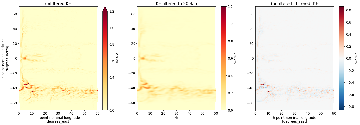
We observe the strongest smoothing at the high latitudes, in the ACC. This is because we used a filter with fixed filter scale. At high latitudes, the grid spacing is the smallest (scroll back up to our plots of dxw and dxs!) and the gap between the grid spacing and the filter scale is the largest.

Filtering with spatially-varying filter scale

We now want to vary the filter scale over our NeverWorld2 domain. In this example, we define the local filter scale equal to the local first baroclinic deformation radius $L_d$, time-averaged over the length of our simulation. Here is the time-averaged deformation radius.

ds['Rd1'].mean(dim='time').plot(figsize=(6,7), vmin=0, cmap='YlGn');

/glade/work/noraloose/my_npl_clone_20201220/lib/python3.7/site-packages/dask/array/numpy_compat.py:40: RuntimeWarning: invalid value encountered in true_divide
  x = np.divide(x1, x2, out)

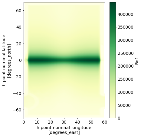
The maximum deformation radius is about 446 km:

L_max = ds['Rd1'].mean(dim='time').max(dim=['yh','xh']).values
L_max

/glade/work/noraloose/my_npl_clone_20201220/lib/python3.7/site-packages/dask/array/numpy_compat.py:40: RuntimeWarning: invalid value encountered in true_divide
  x = np.divide(x1, x2, out)

array(445500.75, dtype=float32)

As described in the Filter Theory, we set filter_scale equal to the largest desired filter scale in the domain, i.e., equal to the maximum deformation radius.

filter_scale = L_max

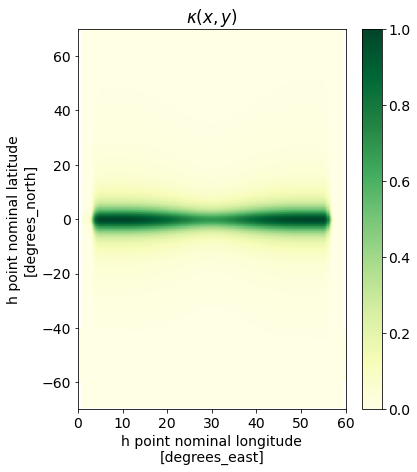
We now set the spatially varying $\kappa$ as $\kappa(x,y) = \frac{L_d(x,y)^2}{L_{max}^2}$.

kappa = ds['Rd1'].mean(dim='time')**2 / L_max**2

fig,ax = plt.subplots(1,1,figsize=(6,7))

kappa.plot(ax=ax, vmin=0, cmap='YlGn', cbar_kwargs={'label': ''})
ax.set(title=r'$\kappa(x,y)$');

/glade/work/noraloose/my_npl_clone_20201220/lib/python3.7/site-packages/dask/array/numpy_compat.py:40: RuntimeWarning: invalid value encountered in true_divide
  x = np.divide(x1, x2, out)

Since we are still using the same grid as in the previous example, we can re-use our grid variables for IRREGULAR_WITH_LAND.

filter_Ld = gcm_filters.Filter(
    filter_scale=filter_scale,
    dx_min=dx_min,
    filter_shape=gcm_filters.FilterShape.GAUSSIAN,
    grid_type=gcm_filters.GridType.IRREGULAR_WITH_LAND,
    grid_vars={
        'wet_mask': wet_mask, 
        'dxw': dxw, 'dyw': dyw, 'dxs': dxs, 'dys': dys, 'area': area, 
        'kappa_w': kappa, 'kappa_s': kappa
    }
)
filter_Ld

Filter(filter_scale=array(445500.75, dtype=float32), dx_min=array(9518.17259783), filter_shape=<FilterShape.GAUSSIAN: 1>, transition_width=3.141592653589793, ndim=2, n_steps=52, grid_type=<GridType.IRREGULAR_WITH_LAND: 5>)

We apply the new filter to our kinetic energy field.

KE_filtered_to_Ld = filter_Ld.apply(ds.KE, dims=['yh', 'xh'])

Plotting the filtered field triggers the computation.

fig,axs = plt.subplots(1,3,figsize=(25,8))

ds.KE.isel(time=time, zl=layer).plot(
    ax=axs[0], 
    vmin=vmin, vmax=vmax, 
    cmap='YlOrRd', cbar_kwargs={'label': 'm2 s-2'}
)
axs[0].set(title='unfiltered KE')

KE_filtered_to_Ld.isel(time=time, zl=layer).plot(
    ax=axs[1], 
    vmin=vmin, vmax=vmax, 
    cmap='YlOrRd', cbar_kwargs={'label': 'm2 s-2'}
)
axs[1].set(title='KE filtered to scale of deformation radius', ylabel='')

(ds.KE - KE_filtered_to_Ld).isel(time=time, zl=layer).plot(
    ax=axs[2], 
    cmap='RdBu_r', cbar_kwargs={'label': 'm2 s-2'}
)
axs[2].set(title='(unfiltered - filtered) KE', ylabel='');

/glade/work/noraloose/my_npl_clone_20201220/lib/python3.7/site-packages/dask/array/numpy_compat.py:40: RuntimeWarning: invalid value encountered in true_divide
  x = np.divide(x1, x2, out)
/glade/work/noraloose/my_npl_clone_20201220/lib/python3.7/site-packages/dask/array/numpy_compat.py:40: RuntimeWarning: invalid value encountered in true_divide
  x = np.divide(x1, x2, out)

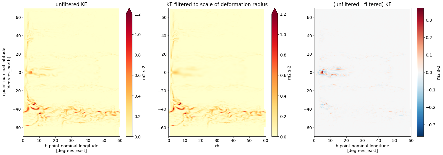
In contrast to our previous example, the strongest smoothing occurs now close to the equator. This is because close to the equator, the local filter scale (i.e. the local deformation radius) is much larger than at high latitudes.

Anisotropic filtering

Next, we want to use anisotropic filters that have different filter scales in the zonal and meridional directions. Note that zonal and meridional directions are aligned with our NeverWorld2 (spherical) grid directions. The theory behind anisotropic filtering is described here.

The first anisotropic filter has a filter scale of 300 km in zonal direction, and 30 km in meridional direction. We will name this filter filter_aniso_y.

filter_scale = 300000
kappa_w = xr.ones_like(dxw)
kappa_s = 0.01 * xr.ones_like(dxs)

filter_aniso_y = gcm_filters.Filter(
    filter_scale=filter_scale,
    dx_min=dx_min,
    filter_shape=gcm_filters.FilterShape.GAUSSIAN,
    grid_type=gcm_filters.GridType.IRREGULAR_WITH_LAND,
    grid_vars={
        'wet_mask': wet_mask, 
        'dxw': dxw, 'dyw': dyw, 'dxs': dxs, 'dys': dys, 'area': area, 
        'kappa_w': kappa_w, 'kappa_s': kappa_s
    }
)
filter_aniso_y

Filter(filter_scale=300000, dx_min=array(9518.17259783), filter_shape=<FilterShape.GAUSSIAN: 1>, transition_width=3.141592653589793, ndim=2, n_steps=35, grid_type=<GridType.IRREGULAR_WITH_LAND: 5>)

The second anisotropic filter has a filter scale of 30 km in zonal direction, and 300 km in meridional direction. We will name this filter filter_aniso_x.

filter_scale = 300000
kappa_w = 0.01 * xr.ones_like(dxw)
kappa_s = xr.ones_like(dxs)

filter_aniso_x = gcm_filters.Filter(
    filter_scale=filter_scale,
    dx_min=dx_min,
    filter_shape=gcm_filters.FilterShape.GAUSSIAN,
    grid_type=gcm_filters.GridType.IRREGULAR_WITH_LAND,
    grid_vars={
        'wet_mask': wet_mask, 
        'dxw': dxw, 'dyw': dyw, 'dxs': dxs, 'dys': dys, 'area': area, 
        'kappa_w': kappa_w, 'kappa_s': kappa_s
    }
)
filter_aniso_x

Filter(filter_scale=300000, dx_min=array(9518.17259783), filter_shape=<FilterShape.GAUSSIAN: 1>, transition_width=3.141592653589793, ndim=2, n_steps=35, grid_type=<GridType.IRREGULAR_WITH_LAND: 5>)

We filter our kinetic energy field with both filters.

KE_filtered_aniso_y = filter_aniso_y.apply(ds.KE, dims=['yh', 'xh'])
KE_filtered_aniso_x = filter_aniso_x.apply(ds.KE, dims=['yh', 'xh'])

Here is the result of our two filtering operations.

fig,axs = plt.subplots(1,3,figsize=(25,8))

ds.KE.isel(time=time, zl=layer).plot(
    ax=axs[0], 
    vmin=vmin, vmax=vmax, 
    cmap='YlOrRd', cbar_kwargs={'label': 'm2 s-2'}
)
axs[0].set(title='unfiltered KE')

KE_filtered_aniso_y.isel(time=time, zl=layer).plot(
    ax=axs[1], 
    vmin=vmin, vmax=vmax, 
    cmap='YlOrRd', cbar_kwargs={'label': 'm2 s-2'}
)
axs[1].set(title='KE filtered to 300km zonally, 30km meridionally', ylabel='')

KE_filtered_aniso_x.isel(time=time, zl=layer).plot(
    ax=axs[2], 
    vmin=vmin, vmax=vmax, 
    cmap='YlOrRd', cbar_kwargs={'label': 'm2 s-2'}
)
axs[2].set(title='KE filtered to 30km zonally, 300km meridionally', ylabel='');

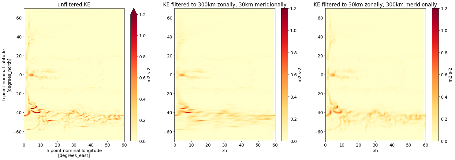
The filtered fields show a clear zonally (middle) and meridionally (right) smooth structure.

Filtering with a fixed factor

In the next example, our goal is to use a filter that removes scales smaller than 10 times the local grid scale. We call this filter type a fixed factor filter. To achieve this, we will combine aspects from the previous 2 examples, and use a spatially-varying & anisotropic filter.

First, we need to know the maximum grid spacing.

dx_max = max(dxw.max(),dyw.max(),dxs.max(),dys.max())
dx_max = dx_max.values
dx_max

array(27829.27492305)

As explained in the Filter Theory and Section 2.6 in Grooms et al. (2021), we set filter_scale, kappa_w and kappa_s as follows.

filter_scale = 10 * dx_max
kappa_w = dxw * dxw / (dx_max * dx_max)
kappa_s = dys * dys / (dx_max * dx_max)

filter_fixed_factor = gcm_filters.Filter(
    filter_scale=filter_scale,
    dx_min=dx_min,
    filter_shape=gcm_filters.FilterShape.GAUSSIAN,
    grid_type=gcm_filters.GridType.IRREGULAR_WITH_LAND,
    grid_vars={
        'wet_mask': wet_mask, 
        'dxw': dxw, 'dyw': dyw, 'dxs': dxs, 'dys': dys, 'area': area, 
        'kappa_w': kappa_w, 'kappa_s': kappa_s
    }
)
filter_fixed_factor

Filter(filter_scale=278292.7492304958, dx_min=array(9518.17259783), filter_shape=<FilterShape.GAUSSIAN: 1>, transition_width=3.141592653589793, ndim=2, n_steps=33, grid_type=<GridType.IRREGULAR_WITH_LAND: 5>)

Note that the number of required steps, n_steps, is 33. (Let’s keep this number in mind for the next example.) But first, we filter kinetic energy as usual.

KE_filtered_fixed_factor = filter_fixed_factor.apply(ds.KE, dims=['yh', 'xh'])

fig,axs = plt.subplots(1,3,figsize=(25,8))

ds.KE.isel(time=time, zl=layer).plot(
    ax=axs[0], 
    vmin=vmin, vmax=vmax, 
    cmap='YlOrRd', cbar_kwargs={'label': 'm2 s-2'}
)
axs[0].set(title='unfiltered KE')

KE_filtered_fixed_factor.isel(time=time, zl=layer).plot(
    ax=axs[1], 
    vmin=vmin, vmax=vmax, 
    cmap='YlOrRd', cbar_kwargs={'label': 'm2 s-2'}
)
axs[1].set(title='KE filtered to 10 times local grid scale', ylabel='')

(ds.KE - KE_filtered_fixed_factor).isel(time=time, zl=layer).plot(
    ax=axs[2], 
    cmap='RdBu_r', cbar_kwargs={'label': 'm2 s-2'}
)
axs[2].set(title='(unfiltered - filtered) KE', ylabel='');

With a fixed factor, we observe smoothing at both low and high latitudes.

Simple fixed factor filter

In our final example, we use an alternative method to filter with a fixed factor of 10. It is more ad hoc than what we did in the previous example, but simpler and faster (especially if you filter large data sets). In Grooms et al. (2021), Section 2.6, this filter is referred to as the simple fixed factor filter. Simple fixed factor filtering operates on a uniform Cartesian grid with dx = dy = 1 that is being transformed from the original locally orthogonal grid.

filter_scale = 10
dx_min = 1

The REGULAR_WITH_LAND_AREA_WEIGHTED grid type matches our data and is appropriate for simple fixed factor filtering. This simple Laplacian requires the following arguments.

gcm_filters.required_grid_vars(gcm_filters.GridType.REGULAR_WITH_LAND_AREA_WEIGHTED)

['area', 'wet_mask']

We create our simple fixed factor filter.

filter_simple_fixed_factor = gcm_filters.Filter(
    filter_scale=filter_scale,
    dx_min=dx_min,
    filter_shape=gcm_filters.FilterShape.GAUSSIAN,
    grid_type=gcm_filters.GridType.REGULAR_WITH_LAND_AREA_WEIGHTED,
    grid_vars={'area': area, 'wet_mask': wet_mask}
)
filter_simple_fixed_factor

Filter(filter_scale=10, dx_min=1, filter_shape=<FilterShape.GAUSSIAN: 1>, transition_width=3.141592653589793, ndim=2, n_steps=11, grid_type=<GridType.REGULAR_WITH_LAND_AREA_WEIGHTED: 4>)

The number of required steps, n_steps, is now only 11. (It was 33 in the previous example.)

KE_filtered_simple_fixed_factor = filter_simple_fixed_factor.apply(ds.KE, dims=['yh', 'xh'])

Let’s compare the result from the simple fixed factor filter with the more complex (and correct) fixed factor filter from the previous example.

fig,axs = plt.subplots(1,3,figsize=(25,8))

KE_filtered_fixed_factor.isel(time=time, zl=layer).plot(
    ax=axs[0], 
    cmap='YlOrRd', cbar_kwargs={'label': 'm2 s-2'}
)
axs[0].set(title='filtered with fixed factor')

KE_filtered_simple_fixed_factor.isel(time=time, zl=layer).plot(
    ax=axs[1], 
    cmap='YlOrRd', cbar_kwargs={'label': 'm2 s-2'}
)
axs[1].set(title='filtered with fixed factor (simple)', ylabel='')

(KE_filtered_fixed_factor - KE_filtered_simple_fixed_factor).isel(time=time, zl=layer).plot(
    ax=axs[2],
    cbar_kwargs={'label': 'm2 s-2'}    
)
axs[2].set(title='difference', ylabel='');

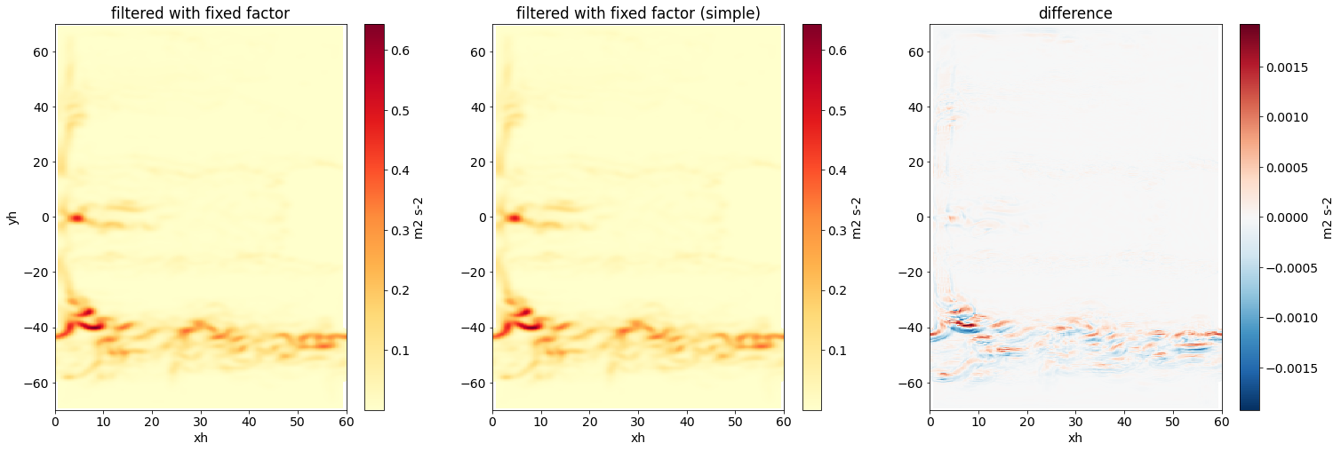
There are differences in the two filtered fields due to the simplicity of the simple fixed factor filter, but the differences are relatively small.