Example: Viscosity-based filtering with vector Laplacians#
In this tutorial, we use viscosity-based filters to filter a velocity field $(u,v)$ on a curvilinear grid. The viscosity-based filter uses a vector Laplacian (rather than a scalar Laplacian).
import gcm_filters
import numpy as np
import xarray as xr
Here are all grid types that we have available.
list(gcm_filters.GridType)
[<GridType.REGULAR: 1>,
 <GridType.REGULAR_AREA_WEIGHTED: 2>,
 <GridType.REGULAR_WITH_LAND: 3>,
 <GridType.REGULAR_WITH_LAND_AREA_WEIGHTED: 4>,
 <GridType.IRREGULAR_WITH_LAND: 5>,
 <GridType.MOM5U: 6>,
 <GridType.MOM5T: 7>,
 <GridType.TRIPOLAR_REGULAR_WITH_LAND_AREA_WEIGHTED: 8>,
 <GridType.TRIPOLAR_POP_WITH_LAND: 9>,
 <GridType.VECTOR_C_GRID: 10>]
From this list, only the VECTOR_C_GRID has a vector Laplacian. All other grid types operate with scalar Laplacians. As the name suggests, the VECTOR_C_GRID works for vector fields that are defined on an Arakawa C-grid, where the u-component is defined at the center of the eastern cell edge, and the v-component at the center of the northern cell edge.
0.1 degree MOM6 data#
We are working with MOM6 data from a 0.1 degree simulation on an Arakawa C-grid. The VECTOR_C_GRID type is therefore suitable for our data!
import pooch

fname = pooch.retrieve(
    url="doi:10.6084/m9.figshare.14718462.v1/MOM6_surf_vels.0.1degree.nc",
    known_hash="md5:99a05ca83f9560fda85ca509a66aafd7",
)
ds = xr.open_dataset(fname)
ds
<xarray.Dataset>
Dimensions:   (xq: 3600, nv: 2, time: 31, xh: 3600, yh: 2400, yq: 2400)
Coordinates:
  * xq        (xq) float64 -109.9 -109.8 -109.7 -109.6 ... -110.2 -110.1 -110.0
  * nv        (nv) float64 1.0 2.0
  * time      (time) object 0022-01-01 12:00:00 ... 0022-01-31 12:00:00
  * xh        (xh) float64 -109.9 -109.8 -109.8 -109.7 ... -110.2 -110.2 -110.1
  * yh        (yh) float64 -78.47 -78.43 -78.39 -78.35 ... 89.88 89.92 89.97
  * yq        (yq) float64 -78.45 -78.41 -78.37 -78.32 ... 89.85 89.9 89.95 90.0
Data variables: (12/23)
    SSU       (yh, xq) float32 ...
    SSV       (yq, xh) float32 ...
    geolon    (yh, xh) float32 ...
    geolon_u  (yh, xq) float32 ...
    geolon_v  (yq, xh) float32 ...
    geolat    (yh, xh) float32 ...
    ...        ...
    wet_v     (yq, xh) float32 ...
    area_t    (yh, xh) float32 ...
    area_u    (yh, xq) float32 ...
    area_v    (yq, xh) float32 ...
    dxBu      (yq, xq) float64 ...
dyBu (yq, xq) float64 ...Preparing the grid info#
These are the grid variables that our vector Laplacian needs to know.
gcm_filters.required_grid_vars(gcm_filters.GridType.VECTOR_C_GRID)
['wet_mask_t',
 'wet_mask_q',
 'dxT',
 'dyT',
 'dxCu',
 'dyCu',
 'dxCv',
 'dyCv',
 'dxBu',
 'dyBu',
 'area_u',
 'area_v',
 'kappa_iso',
 'kappa_aniso']
In the next cell, we swap the xq and yq dimensions to xh and yh. It is important to note that we do this swapping only because gcm-filters requires all input variables to have the same dimensions, even though the Laplacian assumes that the grid variables are staggered. In other words, we do not actually move the data to xh, yh grid points!
# grid info centered at T-points
wet_mask_t = ds.wet
dxT = ds.dxT
dyT = ds.dyT
# grid info centered at U-points
dxCu = ds.dxCu.swap_dims({"xq": "xh"})
dyCu = ds.dyCu.swap_dims({"xq": "xh"})
area_u = dxCu * dyCu
# grid info centered at V-points
dxCv = ds.dxCv.swap_dims({"yq": "yh"})
dyCv = ds.dyCv.swap_dims({"yq": "yh"})
area_v = dxCv * dyCv
# grid info centered at vorticity points
wet_mask_q = ds.wet_c.swap_dims({"xq": "xh", "yq": "yh"})
dxBu = ds.dxBu.swap_dims({"xq": "xh", "yq": "yh"})
dyBu = ds.dyBu.swap_dims({"xq": "xh", "yq": "yh"})
Next, we compute the minimum and maximum grid spacing.
dx_min = min(dxT.where(wet_mask_t).min(), dyT.where(wet_mask_t).min())
dx_min = dx_min.values
dx_min
array(2245.78271484)
dx_max = max(dxT.max(), dyT.max(), dxCu.max(), dyCu.max(), dxCv.max(), dyCv.max(), dxBu.max(), dyBu.max())
dx_max = dx_max.values
dx_max
array(11260.51171875)
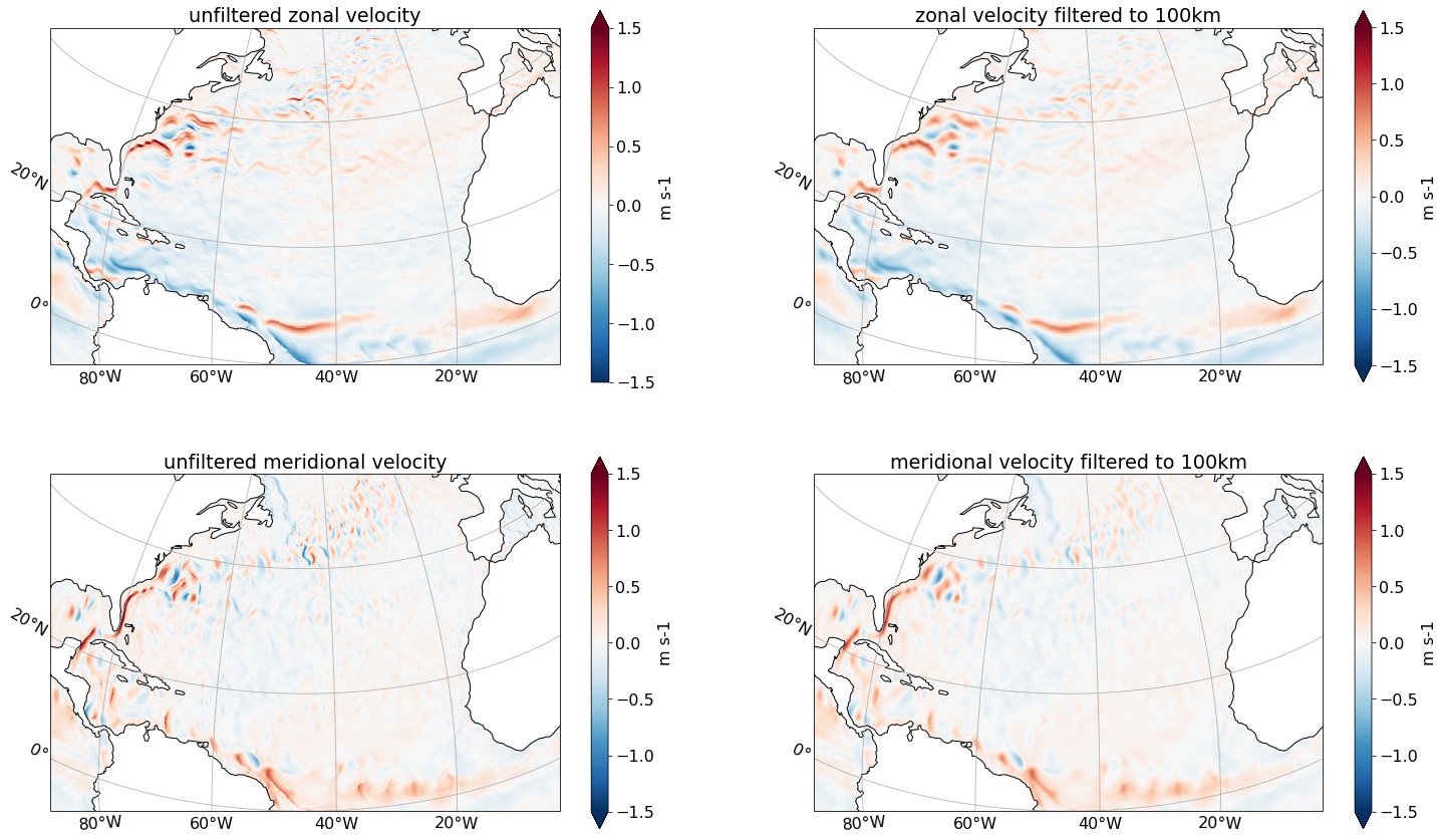
Viscosity-based filtering with fixed length scale#
First, we want to filter velocity with a fixed filter length scale of 100 km. That is, we use a filter that attempts to remove scales smaller than 100 km.
filter_scale = 100000
Since we don’t want to vary the filter scale spatially and we are happy with an isotropic filter, we set kappa_iso equal to 1 and kappa_aniso equal to 0 over the full domain.
kappa_iso = xr.ones_like(dxT)
kappa_aniso = xr.zeros_like(dyT)
Creating the filter#
We now create our filter.
filter_visc_100km = gcm_filters.Filter(
    filter_scale=filter_scale,
    dx_min=dx_min,
    filter_shape=gcm_filters.FilterShape.GAUSSIAN,
    grid_type=gcm_filters.GridType.VECTOR_C_GRID,
    grid_vars={
        'wet_mask_t': wet_mask_t, 'wet_mask_q': wet_mask_q,
        'dxT': dxT, 'dyT': dyT,
        'dxCu': dxCu, 'dyCu': dyCu, 'area_u': area_u,
        'dxCv': dxCv, 'dyCv': dyCv, 'area_v': area_v,
        'dxBu': dxBu, 'dyBu': dyBu,
        'kappa_iso': kappa_iso, 'kappa_aniso': kappa_aniso
    }
)
filter_visc_100km
Filter(filter_scale=100000, dx_min=array(2245.78271484), filter_shape=<FilterShape.GAUSSIAN: 1>, transition_width=3.141592653589793, ndim=2, n_steps=49, grid_type=<GridType.VECTOR_C_GRID: 10>)
Filtering velocity#
We now filter our velocity vector field. In contrast to the diffusion-based filters, the viscosity-based filter takes a vector field (here: $(u,v)$) as input and returns a vector field.
ds_tmp = xr.Dataset()  # temporary dataset with swapped dimensions
ds_tmp['u'] = ds['SSU']
ds_tmp['v'] = ds['SSV']
ds_tmp['u'] = ds_tmp['u'].swap_dims({'xq':'xh'})
ds_tmp['v'] = ds_tmp['v'].swap_dims({'yq':'yh'})
ds_tmp.u
<xarray.DataArray 'u' (yh: 2400, xh: 3600)>
[8640000 values with dtype=float32]
Coordinates:
  * yh       (yh) float64 -78.47 -78.43 -78.39 -78.35 ... 89.88 89.92 89.97
  * xh       (xh) float64 -109.9 -109.8 -109.8 -109.7 ... -110.2 -110.2 -110.1
Attributes:
    long_name:      Sea Surface Zonal Velocity
    units:          m s-1
    cell_methods:   yh:mean xq:point time: mean
    time_avg_info:  average_T1,average_T2,average_DT
interp_method: noneds_tmp.v
<xarray.DataArray 'v' (yh: 2400, xh: 3600)>
[8640000 values with dtype=float32]
Coordinates:
  * yh       (yh) float64 -78.47 -78.43 -78.39 -78.35 ... 89.88 89.92 89.97
  * xh       (xh) float64 -109.9 -109.8 -109.8 -109.7 ... -110.2 -110.2 -110.1
Attributes:
    long_name:      Sea Surface Meridional Velocity
    units:          m s-1
    cell_methods:   yq:point xh:mean time: mean
    time_avg_info:  average_T1,average_T2,average_DT
interp_method: none# apply the filter and compute
%time (u_filtered, v_filtered) = filter_visc_100km.apply_to_vector(ds_tmp.u, ds_tmp.v, dims=['yh', 'xh'])
CPU times: user 32 s, sys: 17.9 s, total: 49.8 s
Wall time: 50 s
We now swap back the dimensions.
ds_tmp['u_filtered'] = u_filtered
ds_tmp['u_filtered'] = ds_tmp['u_filtered'].swap_dims({'xh':'xq'})

ds_tmp['v_filtered'] = v_filtered
ds_tmp['v_filtered'] = ds_tmp['v_filtered'].swap_dims({'yh':'yq'})
Plotting#
import matplotlib.pyplot as plt
import matplotlib.pylab as pylab
params = {'font.size': 16}
pylab.rcParams.update(params)
import matplotlib.ticker as mticker
import cartopy.crs as ccrs
To be able to plot unfiltered and filtered fields using true longitude and latitude, we need to make geolon/geolat coordinates of our xarray.Datasets.
u = ds['SSU'].where(ds.wet_u).assign_coords({'geolat': ds['geolat_u'], 'geolon': ds['geolon_u']})
v = ds['SSV'].where(ds.wet_v).assign_coords({'geolat': ds['geolat_v'], 'geolon': ds['geolon_v']})
u_filtered = ds_tmp.u_filtered.where(ds.wet_u).assign_coords({'geolat': ds['geolat_u'], 'geolon': ds['geolon_u']})
v_filtered = ds_tmp.v_filtered.where(ds.wet_v).assign_coords({'geolat': ds['geolat_v'], 'geolon': ds['geolon_v']})
%%time
# plotting

vmax = 1.5
central_lon = -45
central_lat = 30

fig,axs = plt.subplots(2,2,figsize=(25,15),subplot_kw={'projection':ccrs.Orthographic(central_lon, central_lat)})

u.plot(
    ax=axs[0,0], x='geolon', y='geolat', vmin=-vmax, vmax=vmax,
    cmap='RdBu_r', cbar_kwargs={'label': 'm s-1'},
    transform=ccrs.PlateCarree()
)
v.plot(
    ax=axs[1,0], x='geolon', y='geolat', vmin=-vmax, vmax=vmax,
    cmap='RdBu_r', cbar_kwargs={'label': 'm s-1'},
    transform=ccrs.PlateCarree()
)
u_filtered.plot(
    ax=axs[0,1], x='geolon', y='geolat', vmin=-vmax, vmax=vmax,
    cmap='RdBu_r', cbar_kwargs={'label': 'm s-1'},
    transform=ccrs.PlateCarree()
)
v_filtered.plot(
    ax=axs[1,1], x='geolon', y='geolat', vmin=-vmax, vmax=vmax,
    cmap='RdBu_r', cbar_kwargs={'label': 'm s-1'},
    transform=ccrs.PlateCarree()
)

axs[0,0].set(title='unfiltered zonal velocity')
axs[0,1].set(title='zonal velocity filtered to 100km')
axs[1,0].set(title='unfiltered meridional velocity')
axs[1,1].set(title='meridional velocity filtered to 100km')

for ax in axs.flatten():
    ax.coastlines()
    ax.set_extent([-90, 0, 0, 50], crs=ccrs.PlateCarree())
    gl = ax.gridlines(draw_labels=True)
    gl.xlocator = mticker.FixedLocator([-80,-60,-40,-20])
    gl.ylocator = mticker.FixedLocator([0,20,40,60])
    gl.top_labels = False
    gl.right_labels = False
/glade/work/noraloose/my_npl_clone/lib/python3.7/site-packages/cartopy/mpl/geoaxes.py:1598: UserWarning: The input coordinates to pcolormesh are interpreted as cell centers, but are not monotonically increasing or decreasing. This may lead to incorrectly calculated cell edges, in which case, please supply explicit cell edges to pcolormesh.
  shading=shading)
CPU times: user 11.2 s, sys: 1.18 s, total: 12.4 s
Wall time: 12.7 s
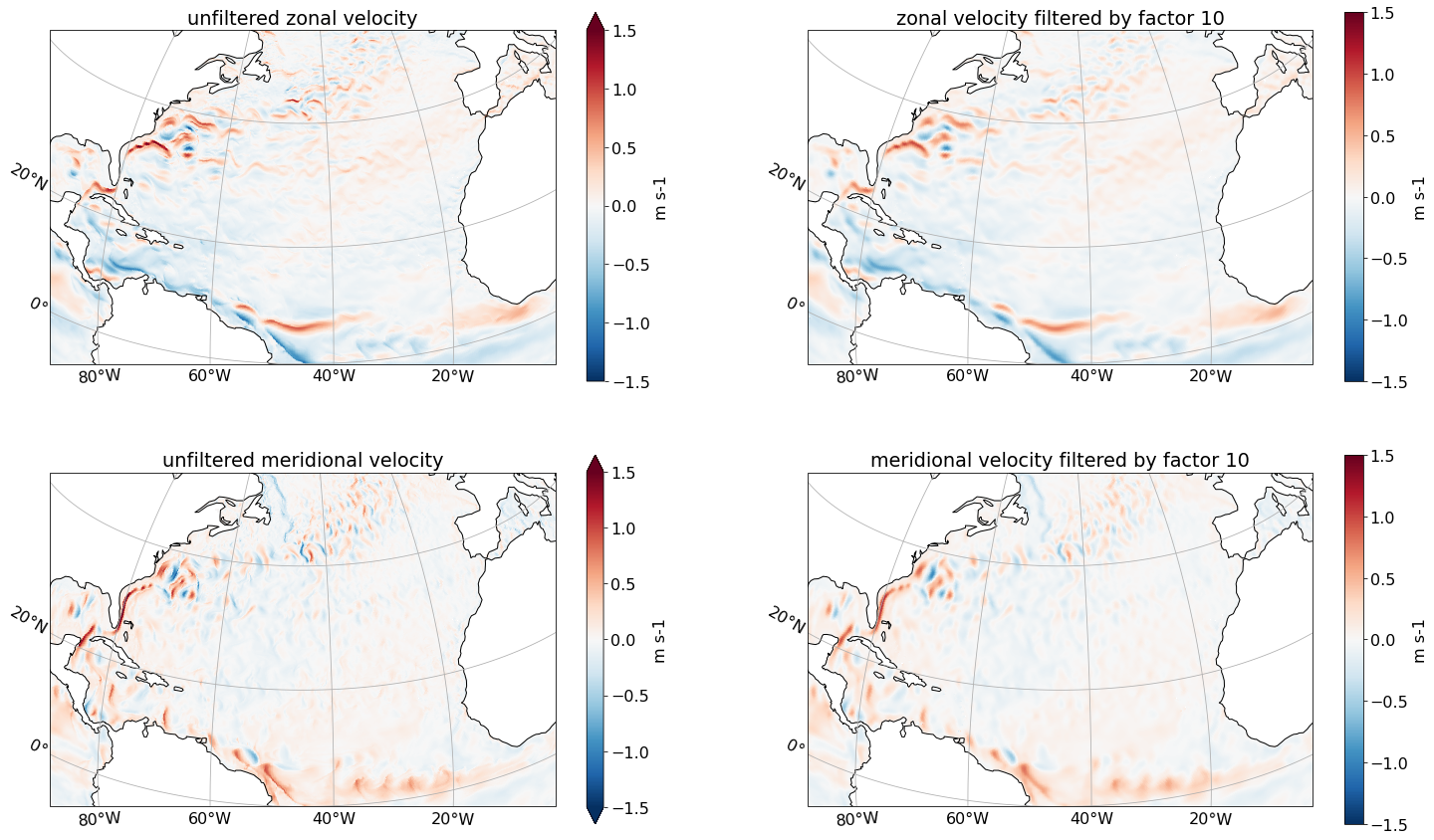
Viscosity-based filtering with fixed filter factor#
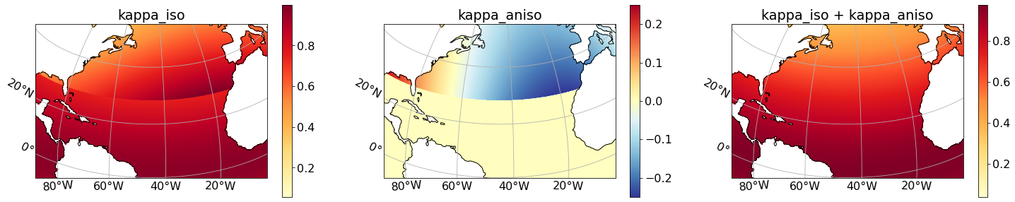
In our second example, we want to filter velocity with a fixed filter factor of 10. That is, our goal is to use a filter that removes scales smaller than 10 times the local grid scale.
The fixed factor filter is a spatially-varying & anisotropic filter. Consistent with the MOM6 implementation of anisotropic viscosity, the conventions for the VECTOR_C_GRID Laplacian are:
kappa_isois the isotropic viscosity,kappa_anisois the additive anisotropy that is aligned with x-direction,
resulting in kappa_x = kappa_iso + kappa_aniso and kappa_y = kappa_iso. Anisotropy in an arbitrary direction (not aligned with the grid directions) is not yet implemented for VECTOR_C_GRID, but could be added mimicking the implementation in MOM6 (following Smith and McWilliams, 2003).
To filter with a fixed factor of 10, we need the filter scale to be equal to ten times $dx_{max}$, together with $\kappa_x = dx^2/dx_{max}^2$ and $\kappa_y = dy^2/dx_{max}^2$, where $dx_{max}$ is the minimum grid spacing in the domain. (See the Filter Theory or Section 2.6 in Grooms et al. (2021) for more details).
filter_scale = 10 * dx_max
kappa_iso = dyCv * dyCv / (dx_max * dx_max)
kappa_aniso = dxCu * dxCu / (dx_max * dx_max) - dyCv * dyCv / (dx_max * dx_max)
The filter needs: $0 < \kappa_{iso} \leq 1$ and $0 < \kappa_{iso} + \kappa_{aniso} \leq 1$. These requirements are satisfied as shown in the next plot.
kappa_iso = kappa_iso.where(wet_mask_t).assign_coords({'geolat': ds['geolat'], 'geolon': ds['geolon']})
kappa_aniso = kappa_aniso.where(wet_mask_t).assign_coords({'geolat': ds['geolat'], 'geolon': ds['geolon']})
%%time

fig,axs = plt.subplots(1,3,figsize=(25,5),subplot_kw={'projection':ccrs.Orthographic(central_lon, central_lat)})

kappa_iso.plot(
    ax=axs[0], x='geolon', y='geolat', cmap='YlOrRd', cbar_kwargs={'label': ''},
    transform=ccrs.PlateCarree()
)
kappa_aniso.plot(
    ax=axs[1], x='geolon', y='geolat', cmap='RdYlBu_r', cbar_kwargs={'label': ''},
    transform=ccrs.PlateCarree()
)
(kappa_iso + kappa_aniso).plot(
    ax=axs[2], x='geolon', y='geolat', cmap='YlOrRd', cbar_kwargs={'label': ''},
    transform=ccrs.PlateCarree()
)

axs[0].set(title='kappa_iso')
axs[1].set(title='kappa_aniso')
axs[2].set(title='kappa_iso + kappa_aniso')

for ax in axs.flatten():
    ax.coastlines()
    ax.set_extent([-90, 0, 0, 50], crs=ccrs.PlateCarree())
    gl = ax.gridlines(draw_labels=True)
    gl.xlocator = mticker.FixedLocator([-80,-60,-40,-20])
    gl.ylocator = mticker.FixedLocator([0,20,40,60])
    gl.top_labels = False
    gl.right_labels = False
/glade/work/noraloose/my_npl_clone/lib/python3.7/site-packages/cartopy/mpl/geoaxes.py:1598: UserWarning: The input coordinates to pcolormesh are interpreted as cell centers, but are not monotonically increasing or decreasing. This may lead to incorrectly calculated cell edges, in which case, please supply explicit cell edges to pcolormesh.
  shading=shading)
CPU times: user 8.86 s, sys: 947 ms, total: 9.81 s
Wall time: 9.9 s
We now create our fixed factor filter.
filter_fac10 = gcm_filters.Filter(
    filter_scale=filter_scale,
    dx_min=dx_min,
    filter_shape=gcm_filters.FilterShape.GAUSSIAN,
    grid_type=gcm_filters.GridType.VECTOR_C_GRID,
    grid_vars={'wet_mask_t': wet_mask_t, 'wet_mask_q': wet_mask_q,
                'dxT': dxT, 'dyT': dyT,
               'dxCu': dxCu, 'dyCu': dyCu, 'area_u': area_u,
               'dxCv': dxCv, 'dyCv': dyCv, 'area_v': area_v,
               'dxBu': dxBu, 'dyBu': dyBu,
               'kappa_iso': kappa_iso, 'kappa_aniso': kappa_aniso
              }
)
filter_fac10
Filter(filter_scale=112605.1171875, dx_min=array(2245.78271484), filter_shape=<FilterShape.GAUSSIAN: 1>, transition_width=3.141592653589793, ndim=2, n_steps=56, grid_type=<GridType.VECTOR_C_GRID: 10>)
We filter surface velocities with the fixed factor filter.
# apply the filter and compute
%time (u_filtered_fac10, v_filtered_fac10) = filter_fac10.apply_to_vector(ds_tmp.u, ds_tmp.v, dims=['yh', 'xh'])
CPU times: user 36.3 s, sys: 20.2 s, total: 56.5 s
Wall time: 56.6 s
ds_tmp['u_filtered_fac10'] = u_filtered_fac10
ds_tmp['u_filtered_fac10'] = ds_tmp['u_filtered_fac10'].swap_dims({'xh':'xq'})

ds_tmp['v_filtered_fac10'] = v_filtered_fac10
ds_tmp['v_filtered_fac10'] = ds_tmp['v_filtered_fac10'].swap_dims({'yh':'yq'})
u_filtered_fac10 = ds_tmp['u_filtered_fac10'].where(ds.wet_u).assign_coords({'geolat': ds['geolat_u'], 'geolon': ds['geolon_u']})
v_filtered_fac10 = ds_tmp['v_filtered_fac10'].where(ds.wet_v).assign_coords({'geolat': ds['geolat_v'], 'geolon': ds['geolon_v']})
%%time
# plotting

vmax = 1.5
central_lon = -45
central_lat = 30

fig,axs = plt.subplots(2,2,figsize=(25,15),subplot_kw={'projection':ccrs.Orthographic(central_lon, central_lat)})

u.plot(
    ax=axs[0,0], x='geolon', y='geolat', vmin=-vmax, vmax=vmax,
    cmap='RdBu_r', cbar_kwargs={'label': 'm s-1'},
    transform=ccrs.PlateCarree()
)
v.plot(
    ax=axs[1,0], x='geolon', y='geolat', vmin=-vmax, vmax=vmax,
    cmap='RdBu_r', cbar_kwargs={'label': 'm s-1'},
    transform=ccrs.PlateCarree()
)
u_filtered_fac10.plot(
    ax=axs[0,1], x='geolon', y='geolat', vmin=-vmax, vmax=vmax,
    cmap='RdBu_r', cbar_kwargs={'label': 'm s-1'},
    transform=ccrs.PlateCarree()
)
v_filtered_fac10.plot(
    ax=axs[1,1], x='geolon', y='geolat', vmin=-vmax, vmax=vmax,
    cmap='RdBu_r', cbar_kwargs={'label': 'm s-1'},
    transform=ccrs.PlateCarree()
)

axs[0,0].set(title='unfiltered zonal velocity')
axs[0,1].set(title='zonal velocity filtered by factor 10')
axs[1,0].set(title='unfiltered meridional velocity')
axs[1,1].set(title='meridional velocity filtered by factor 10')

for ax in axs.flatten():
    ax.coastlines()
    ax.set_extent([-90, 0, 0, 50], crs=ccrs.PlateCarree())
    gl = ax.gridlines(draw_labels=True)
    gl.xlocator = mticker.FixedLocator([-80,-60,-40,-20])
    gl.ylocator = mticker.FixedLocator([0,20,40,60])
    gl.top_labels = False
    gl.right_labels = False
/glade/work/noraloose/my_npl_clone/lib/python3.7/site-packages/cartopy/mpl/geoaxes.py:1598: UserWarning: The input coordinates to pcolormesh are interpreted as cell centers, but are not monotonically increasing or decreasing. This may lead to incorrectly calculated cell edges, in which case, please supply explicit cell edges to pcolormesh.
  shading=shading)
CPU times: user 11.6 s, sys: 1.18 s, total: 12.7 s
Wall time: 12.8 s
Dealing with symmetric model output#
MOM6 output can come in
Symmetric mode:
len(xq) = len(xh) + 1andlen(yq) = len(yh) + 1; orNon-symmetric mode:
len(xq) = len(xh)andlen(yq) = len(yh),
see also this MOM6 tutorial.
In the examples above, we have worked with MOM6 data in non-symmetric mode. Using gcm-filters with data in symmetric mode would be a bit more complicated because we have to remove the extra padding in the xq and yq dimensions before filtering (and re-add this padding after we are done with filtering). We therefore recommend to transform symmetric data to non-symmetric data before using gcm-filters as follows.
from intake import open_catalog
cat = open_catalog('https://raw.githubusercontent.com/ocean-eddy-cpt/cpt-data/master/catalog.yaml')
list(cat)
['neverworld_five_day_averages',
 'neverworld_quarter_degree_snapshots',
 'neverworld_quarter_degree_averages',
 'neverworld_quarter_degree_static',
 'neverworld_quarter_degree_stats',
 'neverworld_eighth_degree_snapshots',
 'neverworld_eighth_degree_averages',
 'neverworld_eighth_degree_static',
 'neverworld_eighth_degree_stats',
 'neverworld_sixteenth_degree_snapshots',
 'neverworld_sixteenth_degree_averages',
 'neverworld_sixteenth_degree_static',
 'neverworld_sixteenth_degree_stats']
The NeverWorld2 output is saved in symmetric mode: we have len(xq) = len(xh) + 1 and len(yq) = len(yh) + 1.
ds = cat['neverworld_quarter_degree_averages'].to_dask()
ds_static = cat['neverworld_quarter_degree_static'].to_dask()
ds
<xarray.Dataset>
Dimensions:     (time: 100, zl: 15, yh: 560, xq: 241, yq: 561, xh: 240, zi: 16, nv: 2)
Coordinates:
  * nv          (nv) float64 1.0 2.0
  * time        (time) object 0084-05-03 12:00:00 ... 0085-09-18 12:00:00
  * xh          (xh) float64 0.125 0.375 0.625 0.875 ... 59.12 59.38 59.62 59.88
  * xq          (xq) float64 0.0 0.25 0.5 0.75 1.0 ... 59.25 59.5 59.75 60.0
  * yh          (yh) float64 -69.88 -69.62 -69.38 -69.12 ... 69.38 69.62 69.88
  * yq          (yq) float64 -70.0 -69.75 -69.5 -69.25 ... 69.25 69.5 69.75 70.0
  * zi          (zi) float64 1.022e+03 1.023e+03 ... 1.028e+03 1.028e+03
  * zl          (zl) float64 1.023e+03 1.023e+03 ... 1.028e+03 1.028e+03
Data variables: (12/33)
    CAu         (time, zl, yh, xq) float32 dask.array<chunksize=(10, 15, 560, 241), meta=np.ndarray>
    CAv         (time, zl, yq, xh) float32 dask.array<chunksize=(10, 15, 561, 240), meta=np.ndarray>
    KE          (time, zl, yh, xh) float32 dask.array<chunksize=(10, 15, 560, 240), meta=np.ndarray>
    KE_BT       (time, zl, yh, xh) float32 dask.array<chunksize=(10, 15, 560, 240), meta=np.ndarray>
    KE_CorAdv   (time, zl, yh, xh) float32 dask.array<chunksize=(10, 15, 560, 240), meta=np.ndarray>
    KE_adv      (time, zl, yh, xh) float32 dask.array<chunksize=(10, 15, 560, 240), meta=np.ndarray>
    ...          ...
    u           (time, zl, yh, xq) float32 dask.array<chunksize=(10, 15, 560, 241), meta=np.ndarray>
    u_BT_accel  (time, zl, yh, xq) float32 dask.array<chunksize=(10, 15, 560, 241), meta=np.ndarray>
    uh          (time, zl, yh, xq) float32 dask.array<chunksize=(10, 15, 560, 241), meta=np.ndarray>
    v           (time, zl, yq, xh) float32 dask.array<chunksize=(10, 15, 561, 240), meta=np.ndarray>
    v_BT_accel  (time, zl, yq, xh) float32 dask.array<chunksize=(10, 15, 561, 240), meta=np.ndarray>
    vh          (time, zl, yq, xh) float32 dask.array<chunksize=(10, 15, 561, 240), meta=np.ndarray>
Attributes:
    associated_files:  area_t: static.nc
    filename:          averages_00030002.nc
    grid_tile:         N/A
    grid_type:         regular
title: NeverWorld2To transform the symmetric data to non-symmetric data, we simply do the following.
ds = ds.isel(xq = slice(1,None), yq=slice(1,None))
ds_static = ds_static.isel(xq = slice(1,None), yq=slice(1,None))
ds
<xarray.Dataset>
Dimensions:     (time: 100, zl: 15, yh: 560, xq: 240, yq: 560, xh: 240, zi: 16, nv: 2)
Coordinates:
  * nv          (nv) float64 1.0 2.0
  * time        (time) object 0084-05-03 12:00:00 ... 0085-09-18 12:00:00
  * xh          (xh) float64 0.125 0.375 0.625 0.875 ... 59.12 59.38 59.62 59.88
  * xq          (xq) float64 0.25 0.5 0.75 1.0 1.25 ... 59.25 59.5 59.75 60.0
  * yh          (yh) float64 -69.88 -69.62 -69.38 -69.12 ... 69.38 69.62 69.88
  * yq          (yq) float64 -69.75 -69.5 -69.25 -69.0 ... 69.25 69.5 69.75 70.0
  * zi          (zi) float64 1.022e+03 1.023e+03 ... 1.028e+03 1.028e+03
  * zl          (zl) float64 1.023e+03 1.023e+03 ... 1.028e+03 1.028e+03
Data variables: (12/33)
    CAu         (time, zl, yh, xq) float32 dask.array<chunksize=(10, 15, 560, 240), meta=np.ndarray>
    CAv         (time, zl, yq, xh) float32 dask.array<chunksize=(10, 15, 560, 240), meta=np.ndarray>
    KE          (time, zl, yh, xh) float32 dask.array<chunksize=(10, 15, 560, 240), meta=np.ndarray>
    KE_BT       (time, zl, yh, xh) float32 dask.array<chunksize=(10, 15, 560, 240), meta=np.ndarray>
    KE_CorAdv   (time, zl, yh, xh) float32 dask.array<chunksize=(10, 15, 560, 240), meta=np.ndarray>
    KE_adv      (time, zl, yh, xh) float32 dask.array<chunksize=(10, 15, 560, 240), meta=np.ndarray>
    ...          ...
    u           (time, zl, yh, xq) float32 dask.array<chunksize=(10, 15, 560, 240), meta=np.ndarray>
    u_BT_accel  (time, zl, yh, xq) float32 dask.array<chunksize=(10, 15, 560, 240), meta=np.ndarray>
    uh          (time, zl, yh, xq) float32 dask.array<chunksize=(10, 15, 560, 240), meta=np.ndarray>
    v           (time, zl, yq, xh) float32 dask.array<chunksize=(10, 15, 560, 240), meta=np.ndarray>
    v_BT_accel  (time, zl, yq, xh) float32 dask.array<chunksize=(10, 15, 560, 240), meta=np.ndarray>
    vh          (time, zl, yq, xh) float32 dask.array<chunksize=(10, 15, 560, 240), meta=np.ndarray>
Attributes:
    associated_files:  area_t: static.nc
    filename:          averages_00030002.nc
    grid_tile:         N/A
    grid_type:         regular
title: NeverWorld2The data is now in the same format (non-symmetric mode) as in the examples above, and you can start filtering!