Basic Filtering#
The Filter Object#
The core object in GCM-Filters is the gcm_filters.Filter object. Its full documentation below enumerates all possible options.
- gcm_filters.Filter(filter_scale: float, dx_min: float, filter_shape: ~gcm_filters.filter.FilterShape = FilterShape.GAUSSIAN, transition_width: float = 3.141592653589793, ndim: int = 2, n_steps: int = 0, grid_type: ~gcm_filters.kernels.GridType = GridType.REGULAR, grid_vars: dict = <factory>) None[source]#
A class for applying diffusion-based smoothing filters to gridded data.
- Parameters:
filter_scale (float) – The filter scale, which has different meaning depending on filter shape
dx_min (float) – The smallest grid spacing. Should have same units as
filter_scalen_steps (int, optional) – Number of total steps in the filter
n_steps == 0means the number of steps is chosen automaticallyfilter_shape (FilterShape) –
FilterShape.GAUSSIAN: The target filter has shape \(e^{-(k filter_scale)^2/24}\)FilterShape.TAPER: The target filter has target grid scale Lf. Smaller scales are zeroed out. Scales larger thanpi * filter_scale / 2are left as-is. In between is a smooth transition.
transition_width (float, optional) – Width of the transition region in the “Taper” filter. This is a nondimensional parameter. Theoretical minimum is 1; not recommended.
ndim (int, optional) – Laplacian is applied on a grid of dimension ndim
grid_type (GridType) – what sort of grid we are dealing with
grid_vars (dict) – dictionary of extra parameters used to initialize the grid Laplacian
- gcm_filters.filter_spec#
- Type:
FilterSpec
Details related to filter_scale, filter_shape, transition_width, and n_steps can be found in the Filter Theory.
The following sections explain the options for grid_type and grid_vars in more detail.
Grid types#
To define a filter, we need to pick a grid and associated Laplacian that matches our data. The currently implemented grid types are:
In [1]: import gcm_filters

In [2]: list(gcm_filters.GridType)
Out[2]:
[<GridType.REGULAR: 1>,
 <GridType.REGULAR_AREA_WEIGHTED: 2>,
 <GridType.REGULAR_WITH_LAND: 3>,
 <GridType.REGULAR_WITH_LAND_AREA_WEIGHTED: 4>,
 <GridType.IRREGULAR_WITH_LAND: 5>,
 <GridType.MOM5U: 6>,
 <GridType.MOM5T: 7>,
 <GridType.TRIPOLAR_REGULAR_WITH_LAND_AREA_WEIGHTED: 8>,
 <GridType.TRIPOLAR_POP_WITH_LAND: 9>,
 <GridType.VECTOR_C_GRID: 10>,
 <GridType.VECTOR_B_GRID: 11>]
This list will grow as we implement more Laplacians.
The following table provides an overview of these different grid type options: what grid they are suitable for, whether they handle land (i.e., continental boundaries), what boundary condition the Laplacian operators use, and whether they come with a scalar or vector Laplacian. You can also find links to example usages.
|
Grid |
Handles land |
Boundary condition |
Laplacian type |
Example |
|---|---|---|---|---|---|
|
Cartesian grid |
no |
periodic |
Scalar Laplacian |
|
|
Cartesian grid |
yes |
periodic |
Scalar Laplacian |
see below |
|
locally orthogonal grid |
yes |
periodic |
Scalar Laplacian |
Example: Different filter types; Example: Filtering on a tripole grid |
|
Velocity-point on Arakawa B-Grid |
yes |
periodic |
Scalar Laplacian |
|
|
Tracer-point on Arakawa B-Grid |
yes |
periodic |
Scalar Laplacian |
|
|
locally orthogonal grid |
yes |
tripole |
Scalar Laplacian |
|
|
yes |
periodic |
Vector Laplacian |
||
|
no |
periodic |
Vector Laplacian |
Grid types with scalar Laplacians can be used for filtering scalar fields (such as temperature), and grid types with vector Laplacians can be used for filtering vector fields (such as velocity).
Grid types for simple fixed factor filtering#
The remaining grid types are for a special type of filtering: simple fixed factor filtering to achieve a fixed coarsening factor (see also the Filter Theory). If you specify one of the following grid types for your data, gcm_filters will internally transform your original (locally orthogonal) grid to a uniform Cartesian grid with dx = dy = 1, and perform fixed factor filtering on the uniform grid. After this is done, gcm_filters transforms the filtered field back to your original grid.
In practice, this coordinate transformation is achieved by area weighting and deweighting (see Filter Theory). This is why the following grid types have the suffix AREA_WEIGHTED.
|
Grid |
Handles land |
Boundary condition |
Laplacian type |
Example |
|---|---|---|---|---|---|
|
locally orthogonal grid |
no |
periodic |
Scalar Laplacian |
|
|
locally orthogonal grid |
yes |
periodic |
Scalar Laplacian |
Example: Different filter types; Example: Filtering on a tripole grid |
|
locally orthogonal grid |
yes |
tripole |
Scalar Laplacian |
Grid variables#
Each grid type from the above two tables has different grid variables that must be provided as Xarray DataArrays. For example, let’s assume we are on a Cartesian grid (with uniform grid spacing equal to 1), and we want to use the grid type REGULAR_WITH_LAND. To find out what the required grid variables for this grid type are, we can use this utility function.
In [3]: gcm_filters.required_grid_vars(gcm_filters.GridType.REGULAR_WITH_LAND)
Out[3]: ['wet_mask']
wet_mask is a binary array representing the topography on our grid. Here the convention is that the array is 1 in the ocean (“wet points”) and 0 on land (“dry points”).
In [4]: import numpy as np

In [5]: import xarray as xr

In [6]: ny, nx = (128, 256)

In [7]: mask_data = np.ones((ny, nx))

In [8]: mask_data[(ny // 4):(3 * ny // 4), (nx // 4):(3 * nx // 4)] = 0

In [9]: wet_mask = xr.DataArray(mask_data, dims=['y', 'x'])
In [10]: wet_mask.plot()
Out[10]: <matplotlib.collections.QuadMesh at 0x7fefa02f7b60>
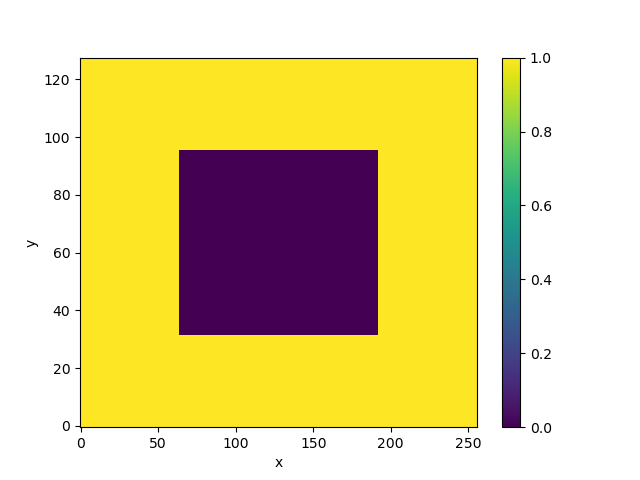
We have made a big island.
Note
Some more complicated grid types require more grid variables.
The units for these variables should be consistent, but no specific system of units is required.
For example, if grid cell edge lengths are defined using kilometers, then the filter scale and dx_min should also be defined using kilometers, and the grid cell areas should be defined in square kilometers.
Creating the Filter Object#
We create a filter object as follows.
In [11]: filter = gcm_filters.Filter(
   ....:     filter_scale=4,
   ....:     dx_min=1,
   ....:     filter_shape=gcm_filters.FilterShape.TAPER,
   ....:     grid_type=gcm_filters.GridType.REGULAR_WITH_LAND,
   ....:     grid_vars={'wet_mask': wet_mask}
   ....: )
   ....:

In [12]: filter
Out[12]: Filter(filter_scale=4, dx_min=1, filter_shape=<FilterShape.TAPER: 2>, transition_width=3.141592653589793, ndim=2, n_steps=np.int64(16), grid_type=<GridType.REGULAR_WITH_LAND: 3>)
The string representation for the filter object in the last line includes some of the parameters it was initiliazed with, to help us keep track of what we are doing. We have created a Taper filter that will filter our data by a fixed factor of 4.
Applying the Filter#
We can now apply the filter object that we created above to some data. Let’s create a random 3D cube of data that matches our grid.
In [13]: nt = 10

In [14]: data = np.random.rand(nt, ny, nx)

In [15]: da = xr.DataArray(data, dims=['time', 'y', 'x'])

In [16]: da
Out[16]:
<xarray.DataArray (time: 10, y: 128, x: 256)> Size: 3MB
array([[[6.56479391e-01, 6.26561375e-01, 8.38712682e-01, ...,
         2.20500164e-01, 3.96733989e-01, 1.70900811e-01],
        [2.87497644e-01, 5.82897857e-01, 1.88574940e-01, ...,
         2.32794018e-01, 4.27377706e-01, 3.70875723e-01],
        [8.45212299e-01, 7.07671799e-01, 8.22491721e-01, ...,
         6.30149934e-01, 8.75789777e-01, 5.05724849e-01],
        ...,
        [2.68097461e-01, 3.89499455e-01, 5.82685822e-01, ...,
         3.00838284e-01, 2.18621708e-01, 9.01159536e-01],
        [9.37585949e-01, 2.35235530e-01, 6.42493463e-01, ...,
         9.11410852e-01, 7.11071334e-01, 5.24753891e-01],
        [7.85135966e-01, 8.64710691e-02, 2.10794603e-01, ...,
         6.99737426e-01, 3.95682212e-01, 4.83034698e-01]],

       [[4.27575767e-01, 9.32011195e-01, 6.24867597e-01, ...,
         9.22295245e-03, 9.69142977e-02, 6.79525533e-01],
        [8.36719027e-01, 4.93672145e-01, 1.82929359e-02, ...,
         4.22208755e-01, 9.69750117e-01, 9.20266826e-02],
        [9.63105791e-02, 3.38785046e-01, 5.29441475e-01, ...,
         9.40099427e-01, 3.85508205e-01, 1.30092969e-01],
...
        [8.86146517e-01, 3.53698286e-01, 6.64101275e-01, ...,
         8.53954049e-02, 1.69925336e-01, 6.26313929e-02],
        [3.57655498e-02, 4.01571025e-01, 8.59244595e-01, ...,
         2.98689534e-01, 1.91369439e-01, 1.95956854e-01],
        [7.52495577e-01, 2.16709451e-01, 8.27380198e-01, ...,
         2.50169206e-01, 4.13168864e-01, 9.09758737e-02]],

       [[3.54102719e-01, 2.47048243e-02, 8.00308843e-01, ...,
         1.03859319e-01, 8.56703882e-01, 9.45689392e-01],
        [4.94965848e-01, 4.47607450e-01, 1.75969538e-01, ...,
         1.32305548e-01, 6.95902526e-01, 9.69904464e-01],
        [3.31182598e-01, 2.19079956e-01, 4.96961335e-01, ...,
         5.24696338e-01, 5.90681323e-01, 7.13700429e-01],
        ...,
        [3.00924293e-01, 5.86303041e-01, 2.66741790e-02, ...,
         5.51880593e-01, 3.05989615e-01, 3.89180041e-01],
        [7.46841694e-01, 7.94312451e-01, 6.96754819e-01, ...,
         6.95637535e-02, 4.56704451e-01, 5.92132733e-01],
        [9.54245308e-01, 2.61460615e-01, 6.39772154e-01, ...,
         3.45927738e-01, 9.05641431e-01, 7.24173593e-01]]])
Dimensions without coordinates: time, y, x
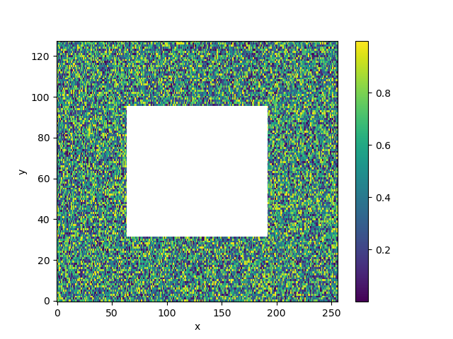
We now mask our data with the wet_mask.
In [17]: da_masked = da.where(wet_mask)
In [18]: da_masked.isel(time=0).plot()
Out[18]: <matplotlib.collections.QuadMesh at 0x7fefa0239590>
Now that we have some data, we can apply our filter. We need to specify which dimension names to apply the filter over. In this case, it is y, x.
Warning
The dimension order matters! Since some filters deal with anisotropic grids, the latitude / y dimension must appear first in order to obtain the correct result. That is not an issue for this simple (isotropic) toy example but needs to be kept in mind for applications on real GCM grids.
In [19]: %time da_filtered = filter.apply(da_masked, dims=['y', 'x'])
CPU times: user 124 ms, sys: 11.9 ms, total: 136 ms
Wall time: 136 ms
In [20]: da_filtered
Out[20]:
<xarray.DataArray (time: 10, y: 128, x: 256)> Size: 3MB
array([[[0.48977607, 0.48990011, 0.49935142, ..., 0.42248709,
         0.4440286 , 0.47614228],
        [0.49785607, 0.52379665, 0.56938794, ..., 0.39441971,
         0.44015597, 0.47721575],
        [0.51531257, 0.54171561, 0.60068928, ..., 0.41265113,
         0.48032708, 0.50912095],
        ...,
        [0.47397591, 0.45794837, 0.43505704, ..., 0.49108779,
         0.47185569, 0.47467684],
        [0.48928537, 0.45049713, 0.40899418, ..., 0.50427706,
         0.49298161, 0.5007156 ],
        [0.49320718, 0.46298425, 0.43475855, ..., 0.47594984,
         0.47774357, 0.49694907]],

       [[0.48047608, 0.49998726, 0.48464081, ..., 0.34255173,
         0.37606193, 0.43086853],
        [0.48648973, 0.48816436, 0.4631941 , ..., 0.41437317,
         0.43337973, 0.46290061],
        [0.52433916, 0.50983809, 0.48100519, ..., 0.53047902,
         0.53298843, 0.53064012],
...
        [0.40451939, 0.47039682, 0.5353055 , ..., 0.48117113,
         0.41562766, 0.37806044],
        [0.41829656, 0.50909584, 0.59134643, ..., 0.41871562,
         0.37424744, 0.36453741],
        [0.46694575, 0.56660259, 0.65424202, ..., 0.3885497 ,
         0.37805387, 0.39711247]],

       [[0.59473841, 0.49024434, 0.41364492, ..., 0.47940277,
         0.59418852, 0.64587706],
        [0.58489827, 0.48235537, 0.41024414, ..., 0.53758766,
         0.62022589, 0.64630256],
        [0.58374794, 0.50707442, 0.45220511, ..., 0.56031658,
         0.61707066, 0.63163602],
        ...,
        [0.58896909, 0.58737373, 0.57762156, ..., 0.36064015,
         0.4759401 , 0.5589558 ],
        [0.60002038, 0.55880812, 0.51990292, ..., 0.36079428,
         0.50112466, 0.59259419],
        [0.60405877, 0.52385022, 0.45937026, ..., 0.40766238,
         0.54769067, 0.62721231]]])
Dimensions without coordinates: time, y, x
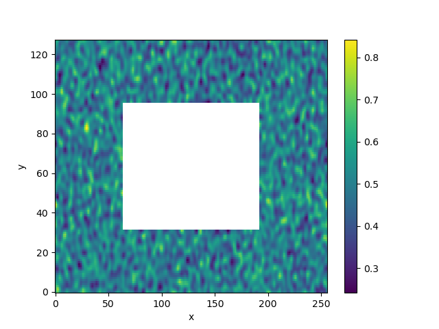
Let’s visualize what the filter did.
In [21]: da_filtered.isel(time=0).plot()
Out[21]: <matplotlib.collections.QuadMesh at 0x7fefa00d3c50>
Using Dask#
Up to now, we have filtered eagerly; when we called .apply, the results were computed immediately and stored in memory.
GCM-Filters is also designed to work seamlessly with Dask array inputs. With dask, we can filter lazily, deferring the filter computations and possibly executing them in parallel.
We can do this with our synthetic data by converting them to dask.
In [22]: da_dask = da_masked.chunk({'time': 2})

In [23]: da_dask
Out[23]:
<xarray.DataArray (time: 10, y: 128, x: 256)> Size: 3MB
dask.array<xarray-<this-array>, shape=(10, 128, 256), dtype=float64, chunksize=(2, 128, 256), chunktype=numpy.ndarray>
Dimensions without coordinates: time, y, x
We now filter our data lazily.
In [24]: da_filtered_lazy = filter.apply(da_dask, dims=['y', 'x'])

In [25]: da_filtered_lazy
Out[25]:
<xarray.DataArray (time: 10, y: 128, x: 256)> Size: 3MB
dask.array<transpose, shape=(10, 128, 256), dtype=float64, chunksize=(2, 128, 256), chunktype=numpy.ndarray>
Dimensions without coordinates: time, y, x
Nothing has actually been computed yet. We can trigger computation as follows:
In [26]: %time da_filtered_computed = da_filtered_lazy.compute()
CPU times: user 357 ms, sys: 65.7 ms, total: 423 ms
Wall time: 329 ms
Here we got only a very modest speedup because our example data are too small. For bigger data, the performance benefit will be more evident.